01 · The Laplace–Beltrami operator: the engine under SpectralBrain

SpectralBrain tutorial series — notebook 1 of 10.

#	Notebook	You are here
01	The Laplace–Beltrami operator	👈
02	Reading real brains: the I/O layer
03	ShapeDNA: hearing the shape of a hippocampus
04	The Heat Kernel Signature
05	Wave Kernel Signature & Global Point Signature
06	Point clouds & white-matter tracts
07	Functional maps & shape distances
08	Cohorts & vertex-wise statistics
09	Effect sizes, classification, harmonization
10	Bayesian spectral analysis & visualization

Every descriptor in SpectralBrain (ShapeDNA, HKS, WKS, GPS, …) is computed from one object: the spectrum of the Laplace–Beltrami operator (LBO) of a surface. If you understand the LBO, you understand the whole library. This notebook builds that understanding from the ground up, on a real hippocampus.

Learning objectives

1. State the eigenvalue problem \(\Delta\varphi = -\lambda\varphi\) and what eigenvalues/eigenfunctions mean.

2. Compute the LBO spectrum of a real surface with mesh.decompose(k).

3. See why low-index eigenfunctions are smooth and high-index ones oscillate.

4. Verify two deep facts numerically: Weyl’s law and isometry invariance.

1. Shape as vibration

In 1966 Mark Kac asked: “Can one hear the shape of a drum?” A drumhead vibrates at a discrete set of frequencies fixed entirely by its shape. Those frequencies are the eigenvalues of the Laplacian, and the vibration patterns are its eigenfunctions. Spectral shape analysis turns Kac’s question around: we listen to a brain structure’s natural frequencies and use them as a fingerprint of its geometry.

The operator

On a smooth surface \(\mathcal{S}\) with Riemannian metric \(g\), the Laplace–Beltrami operator generalises the familiar Laplacian to curved space:

\[\Delta f = \tfrac{1}{\sqrt{|g|}}\,\partial_i\!\left(\sqrt{|g|}\,g^{ij}\,\partial_j f\right).\]

We seek functions that the operator only rescales — the eigenfunctions \(\varphi_k\):

\[\Delta \varphi_k = -\lambda_k \varphi_k, \qquad 0 = \lambda_0 \le \lambda_1 \le \lambda_2 \le \cdots\]

The non-negative numbers \(\lambda_k\) are squared spatial frequencies: small \(\lambda\) = slow, smooth variation; large \(\lambda\) = rapid oscillation.

The discrete operator (what the computer actually solves)

A triangular mesh has no smooth metric, so SpectralBrain uses the cotangent discretization (Pinkall–Polthier; Meyer et al. 2003). It produces two sparse matrices: a stiffness matrix \(L\) (the discrete \(-\Delta\), built from cotangents of triangle angles) and a mass matrix \(M\) (vertex areas). The eigenproblem becomes generalised:

\[L\,\varphi_k = \lambda_k\, M\,\varphi_k.\]

Crucially, \(L\) and \(M\) depend only on edge lengths and angles — intrinsic quantities. Rotating or translating the brain in space does not change them, so the spectrum is invariant to pose. We will prove this to ourselves at the end.

import sys
from pathlib import Path
sys.path.insert(0, str(Path.cwd()))          # so `_tutorial_utils` is importable

import numpy as np
import matplotlib.pyplot as plt
import spectralbrain as sb
from _tutorial_utils import data_path, spectrum_plot

np.set_printoptions(precision=4, suppress=True)

# A real hippocampus: HippUnfold v2 den-8k midthickness surface (subject 03, left).
gii = data_path("hippunfold", "sub03", "hemi-L_space-T1w_den-8k_label-hipp_midthickness.surf.gii")
verts, faces = sb.load_gifti_surface(gii)
hipp = sb.BrainMesh(verts, faces)

print(f"vertices ......... {hipp.n_vertices:,}")
print(f"faces ............ {hipp.n_faces:,}")
print(f"surface area ..... {hipp.surface_area():.1f} mm^2")
print(f"closed surface? .. {hipp.is_closed()}")
print(f"Euler characteristic {hipp.euler_characteristic()}  (genus {hipp.genus()})")

vertices ......... 8,192
faces ............ 16,002
surface area ..... 865.0 mm^2
closed surface? .. False
Euler characteristic 1  (genus 0)

2. Computing the spectrum

mesh.decompose(k) assembles \(L\) and \(M\) and solves the generalised eigenproblem for the smallest \(k\) eigenvalues (the low frequencies carry the shape information; high frequencies are noise — a theme of notebook 10). It returns a decomposition object exposing .eigenvalues \((k,)\) and .eigenvectors \((N, k)\) — the discrete \(\varphi_k\) sampled at the \(N\) vertices.

dec = hipp.decompose(k=100)
print("first 8 eigenvalues:")
print(dec.eigenvalues[:8])
print(f"\nlambda_0 = {dec.eigenvalues[0]:.3e}   (should be ~0: the constant mode)")
print(f"eigenvectors shape: {dec.eigenvectors.shape}   (N_vertices x k)")
print(f"spectral gap (lambda_1 - lambda_0): {dec.spectral_gap:.3e}")

[06/09/26 01:54:26] INFO     Laplacian (cotangent): N=8192, nnz=56578                                              

first 8 eigenvalues:
[0.     0.0058 0.0217 0.03   0.0393 0.0495 0.0587 0.0789]

lambda_0 = 3.990e-17   (should be ~0: the constant mode)
eigenvectors shape: (8192, 100)   (N_vertices x k)
spectral gap (lambda_1 - lambda_0): 1.590e-02

Why \(\lambda_0 = 0\)

A constant function has zero gradient, so \(\Delta(\text{const}) = 0\). The constant is therefore always the first eigenfunction, with eigenvalue exactly \(0\). It carries no shape information and is usually skipped by descriptors. Let us confirm \(\varphi_0\) is (numerically) constant and look at the spectrum.

phi0 = dec.eigenvectors[:, 0]
print(f"phi_0: mean={phi0.mean():.4f}, std={phi0.std():.2e}  -> essentially constant")

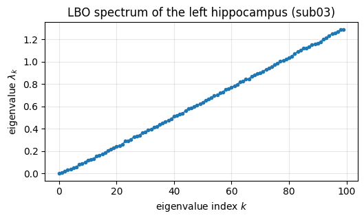
fig, ax = plt.subplots(figsize=(5.4, 3.3))
spectrum_plot(dec.eigenvalues, ax=ax)
ax.set_title("LBO spectrum of the left hippocampus (sub03)")
plt.tight_layout(); plt.show()

phi_0: mean=-0.0340, std=7.21e-16  -> essentially constant

3. Eigenfunctions are vibration modes

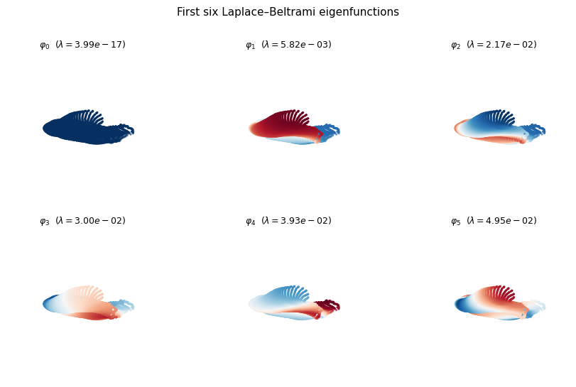
Each \(\varphi_k\) paints a smooth pattern of highs and lows on the surface. The curves where \(\varphi_k = 0\) are its nodal sets (the “still” lines of the drum). As \(k\) grows, the modes oscillate faster and the nodal sets multiply — exactly the behaviour of higher harmonics on an instrument.

Below we colour the mesh vertices by the first six eigenfunctions. Watch the pattern go from a single smooth gradient (\(\varphi_1\), the Fiedler vector) to ever finer oscillations.

def scatter_modes(mesh, dec, n=6, ncols=3):
    V = mesh.vertices
    nrows = int(np.ceil(n / ncols))
    fig = plt.figure(figsize=(ncols * 3.0, nrows * 2.7))
    for i in range(n):
        ax = fig.add_subplot(nrows, ncols, i + 1, projection="3d")
        s = dec.eigenvectors[:, i]
        ax.scatter(V[:, 0], V[:, 1], V[:, 2], c=s, cmap="RdBu_r", s=2,
                   vmin=-np.abs(s).max(), vmax=np.abs(s).max())
        ax.set_title(rf"$\varphi_{{{i}}}$  ($\lambda={dec.eigenvalues[i]:.2e}$)", fontsize=9)
        ax.set_axis_off(); ax.view_init(elev=20, azim=-70)
    fig.suptitle("First six Laplace–Beltrami eigenfunctions", y=1.0, fontsize=11)
    plt.tight_layout(); return fig

scatter_modes(hipp, dec, n=6); plt.show()

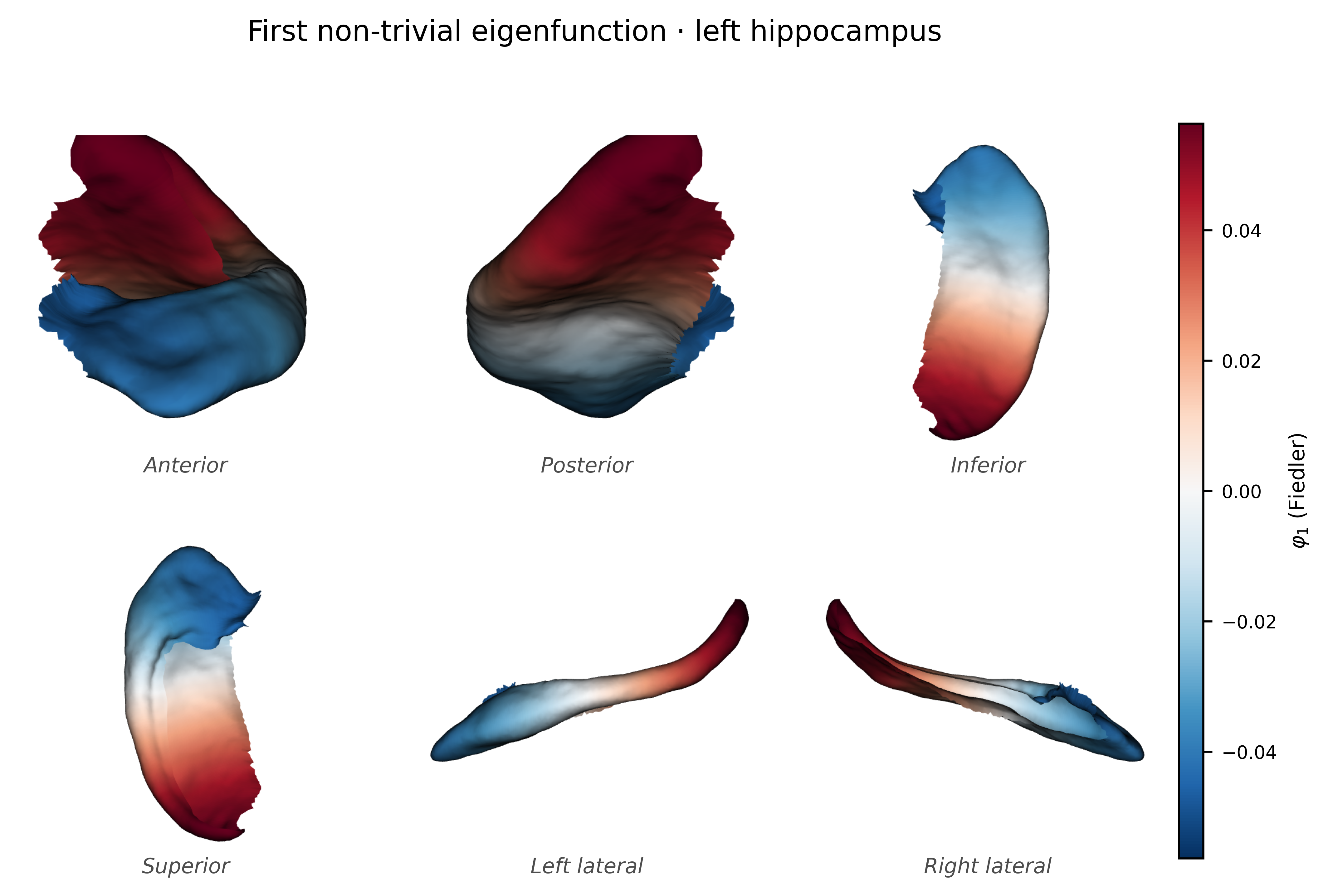
The same low-frequency mode, rendered properly with SpectralBrain’s template-free six-view renderer (the tool we examine in depth in notebook 10). \(\varphi_1\) separates the hippocampal head from the tail — the dominant axis of the shape, recovered automatically from geometry alone.

from spectralbrain.viz import plot_surface_sixview
fig = plot_surface_sixview(hipp, scalars=dec.eigenvectors[:, 1], cmap="RdBu_r",
                           signed=True, scalar_bar_title=r"$\varphi_1$ (Fiedler)",
                           title="First non-trivial eigenfunction · left hippocampus")
plt.show()

2026-06-09 01:54:47.568 (  14.676s) [    7F1F45D63080]vtkXOpenGLRenderWindow.:1460  WARN| bad X server connection. DISPLAY=

4. Weyl’s law: the spectrum counts area

A theorem of Weyl (1911) says the eigenvalues of a 2-D domain grow linearly with their index, at a rate set by the surface area \(A\):

\[\lambda_k \;\sim\; \frac{4\pi}{A}\,k \qquad (k \to \infty).\]

This is why “you can hear the area of a drum.” Let us check it on our hippocampus: plot \(\lambda_k\) against \(k\) and overlay Weyl’s prediction. The agreement is the spectrum literally encoding the surface area we measured in section 1.

k = np.arange(len(dec.eigenvalues))
weyl = 4 * np.pi * k / hipp.surface_area()

fig, ax = plt.subplots(figsize=(5.6, 3.4))
ax.plot(k, dec.eigenvalues, "o-", ms=3, lw=1, label=r"measured $\lambda_k$")
ax.plot(k, weyl, "--", lw=1.6, label=r"Weyl: $4\pi k / A$")
ax.set_xlabel("index $k$"); ax.set_ylabel(r"$\lambda_k$")
ax.set_title("Weyl's law on the hippocampus"); ax.legend(fontsize=9); ax.grid(alpha=0.3)
plt.tight_layout(); plt.show()

slope = np.polyfit(k[10:], dec.eigenvalues[10:], 1)[0]
print(f"fitted slope         : {slope:.3e}")
print(f"Weyl prediction 4pi/A: {4*np.pi/hipp.surface_area():.3e}")

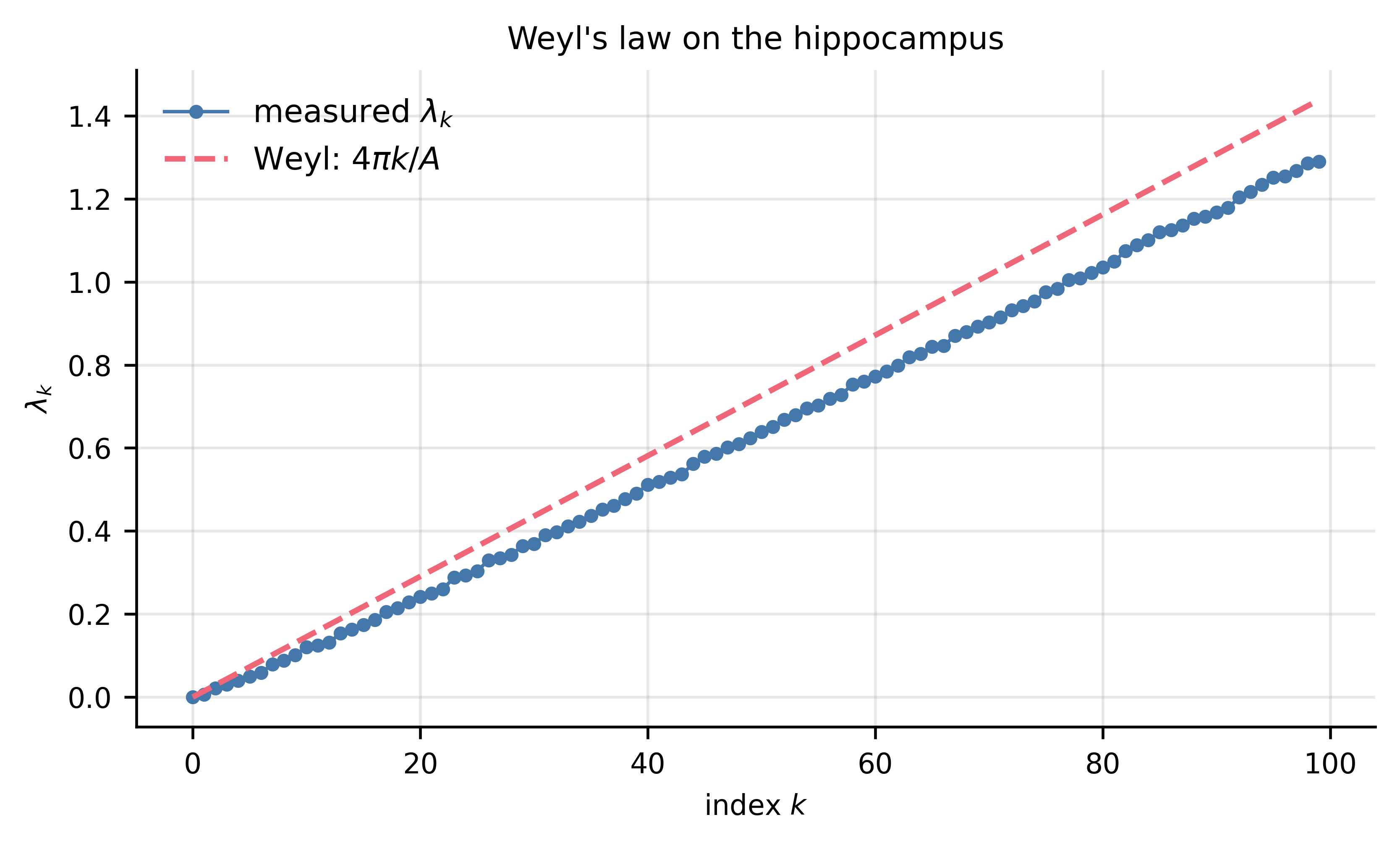
fitted slope         : 1.334e-02
Weyl prediction 4pi/A: 1.453e-02

5. The payoff: isometry invariance

Here is the property that makes spectral descriptors special for neuroimaging. Because \(L\) and \(M\) are built only from edge lengths and angles, any rigid motion of the brain — rotation, translation, reflection — leaves the spectrum unchanged. No registration, no alignment to a template is needed before comparing shapes. Volume- and coordinate-based morphometry cannot say that.

We prove it: take the hippocampus, apply a random rotation and a translation, re-run decompose, and compare the spectra. They should match to numerical precision.

rng = np.random.default_rng(0)
# a random rotation matrix (QR of a random matrix gives an orthonormal R)
R, _ = np.linalg.qr(rng.normal(size=(3, 3)))
if np.linalg.det(R) < 0:
    R[:, 0] *= -1                      # keep it a proper rotation (det +1)
t = rng.normal(scale=50, size=3)       # arbitrary translation

moved = sb.BrainMesh(hipp.vertices @ R.T + t, hipp.faces)
dec_moved = moved.decompose(k=100)

max_diff = np.abs(dec.eigenvalues - dec_moved.eigenvalues).max()
print(f"centroid before : {hipp.vertices.mean(0)}")
print(f"centroid after  : {moved.vertices.mean(0)}")
print(f"max |Δλ| between original and rotated+translated spectrum: {max_diff:.3e}")
assert max_diff < 1e-6, "spectrum should be invariant to rigid motion!"
print("\n✓ The spectrum is invariant to pose — exactly as the theory predicts.")

[06/09/26 01:54:54] INFO     Laplacian (cotangent): N=8192, nnz=56578                                              

centroid before : [-25.0152  12.4943  -4.9732]
centroid after  : [-60.3967 -42.5665  27.9181]
max |Δλ| between original and rotated+translated spectrum: 2.331e-15

✓ The spectrum is invariant to pose — exactly as the theory predicts.

Exercises

1. Resolution vs cost. Time hipp.decompose(k) for k in [25, 50, 100, 200] (use %timeit or time.perf_counter). How does runtime scale? Does \(\lambda_{10}\) change as you add more eigenvalues? (It should not — the small eigenvalues are stable.)

2. Nodal count. For \(\varphi_1,\dots,\varphi_6\), count sign changes per vertex neighbourhood (or simply count connected positive/negative regions). Confirm that higher modes have more nodal domains (Courant’s nodal domain theorem).

3. Left vs right. Load sub03’s right hippocampus, decompose it, and plot both spectra on one axis with spectrum_plot. Where do they diverge — low or high frequencies?

4. Scale sensitivity. Multiply the vertices by 2 (hipp.vertices * 2), re-decompose, and compare eigenvalues. They scale as \(1/\text{area}\), i.e. by \(1/4\). (Notebook 3 shows how ShapeDNA removes this scale factor.)

5. A different structure. Use decompose on a HippUnfold surface from sub04 and compare its spectral gap (dec.spectral_gap) to sub03.

What’s next

You can now turn any surface into a spectrum. But so far we used one pre-loaded hippocampus. Notebook 02 opens the I/O layer: FreeSurfer cortical surfaces, aseg subcortical ROIs, hippocampal subfields, HippUnfold surfaces, and white-matter tracts — the five subjects in tutorials/data/ — and turns each of them into a BrainMesh or BrainPointCloud ready for decompose.