10 · Bayesian spectral analysis & visualization (capstone)#
SpectralBrain tutorial series — notebook 10 of 10. (Previous: effect sizes, classification, harmonization.)
The finale. Frequentist tests gave us p-values and point estimates; the Bayesian layer gives full posterior distributions: honest uncertainty, automatic sparsity, a principled notion of “no meaningful effect,” and normative deviation scores. We close by tying geometry, statistics, and visualization into one workflow.
Learning objectives#
Select predictive descriptors with sparse horseshoe regression.
Compare groups with BEST and judge effects against a region of practical equivalence (ROPE).
Build a Gaussian-process normative model and read per-subject deviation z-scores.
Render a result back onto the anatomy, completing the pipeline.
The feature/outcome cohort is synthetic and clearly labelled, with planted structure so the models have something to recover. MCMC uses short chains for speed; raise
draws/tunefor real analyses.
import sys
from pathlib import Path
sys.path.insert(0, str(Path.cwd()))
import numpy as np, matplotlib.pyplot as plt
import spectralbrain as sb
import spectralbrain.statistics as st
from _tutorial_utils import data_path

rng = np.random.default_rng(11)
n, p = 60, 8
X = rng.normal(size=(n, p))                       # p spectral-descriptor summaries per subject
true_beta = np.array([1.6, 0, 0, -1.1, 0, 0, 0, 0])
y = X @ true_beta + rng.normal(0, 0.5, n)         # an outcome driven by features 0 and 3
group = (rng.random(n) < 0.5).astype(int)         # 0 control, 1 patient
age = rng.uniform(20, 70, n)
print(f"synthetic cohort: {n} subjects, {p} descriptor features (SYNTHETIC — teaching only)")
print(f"outcome truly depends on features 0 and 3")
synthetic cohort: 60 subjects, 8 descriptor features (SYNTHETIC — teaching only)
outcome truly depends on features 0 and 3
1. Sparse horseshoe regression: which descriptors matter?#
With many spectral descriptors, most are probably irrelevant to a given outcome. The horseshoe prior encodes exactly that belief: it pulls most coefficients hard toward zero while letting a few escape to their true value. Formally each coefficient gets its own scale \(\lambda_j\) drawn from a heavy-tailed half-Cauchy, times a global shrinkage \(\tau\):
The posterior should light up features 0 and 3 and flatten the rest.
hs = st.HorseshoeRegression(tau_prior=0.1)
hs.fit(X, y, draws=600, tune=600, chains=2, sampler="auto")
imp = hs.feature_importance()
summ = hs.summary(var_names=["beta"])

fig, ax = plt.subplots(figsize=(5.6, 3.0))
ax.bar(range(p), imp, color=["#9b2d5e" if i in (0, 3) else "#90a4ae" for i in range(p)])
ax.set_xlabel("descriptor feature"); ax.set_ylabel("importance")
ax.set_title("Horseshoe feature importance (planted: 0 and 3)"); ax.grid(alpha=0.3, axis="y")
plt.tight_layout(); plt.show()
print(summ.iloc[:p, :4])
Sampler Progress
Total Chains: 2
Active Chains: 0
Finished Chains: 2
Sampling for now
Estimated Time to Completion: now
| Progress | Draws | Divergences | Step Size | Gradients/Draw |
|---|---|---|---|---|
| 1200 | 34 | 0.23 | 27 | |
| 1200 | 55 | 0.25 | 31 |
[06/09/26 02:30:37] INFO Fitted with nutpie (600 draws × 2 chains).
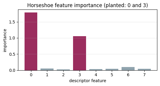
           mean     sd eti94_lb eti94_ub
beta[0]   1.789  0.058      1.7      1.9
beta[1]  -0.043   0.05    -0.15    0.029
beta[2]  -0.004  0.038   -0.088    0.065
beta[3]  -1.059  0.047     -1.1    -0.97
beta[4]   0.023  0.045   -0.049     0.12
beta[5]  -0.031  0.041    -0.12    0.037
beta[6]   0.096  0.055  -0.0024      0.2
beta[7]   0.038  0.043   -0.023     0.13
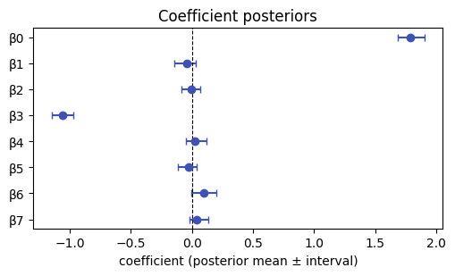
A forest plot of the coefficient posteriors makes the sparsity visible: the relevant features have intervals clear of zero; the rest straddle it.
post = hs.trace_.posterior["beta"].values.reshape(-1, p)   # (samples, p) — version-proof
means = post.mean(0)
lo = np.percentile(post, 3, axis=0); hi = np.percentile(post, 97, axis=0)
fig, ax = plt.subplots(figsize=(5.2, 3.2))
ax.errorbar(means, range(p), xerr=[means - lo, hi - means], fmt="o", color="#3f51b5", capsize=3)
ax.axvline(0, color="k", lw=0.8, ls="--")
ax.set_yticks(range(p)); ax.set_yticklabels([f"β{i}" for i in range(p)])
ax.set_xlabel("coefficient (posterior mean ± interval)"); ax.set_title("Coefficient posteriors")
ax.invert_yaxis(); plt.tight_layout(); plt.show()
2. BEST: group comparison with a ROPE#
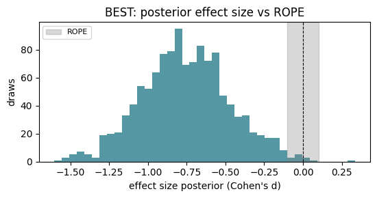
A p-value cannot say “the groups are equivalent.” The Bayesian estimation (BEST) model returns the full posterior of the effect size, and we judge it against a region of practical equivalence (ROPE), a band around zero we deem negligible. The posterior mass below / inside / above the ROPE answers “is there a practically meaningful difference?” directly.
desc_controls = X[group == 0, 0] + rng.normal(0, 0.3, (group == 0).sum())
desc_patients = X[group == 1, 0] + 0.8 + rng.normal(0, 0.3, (group == 1).sum())

best = st.BayesianGroupComparison(rope=(-0.1, 0.1))
best.fit(desc_controls, desc_patients, draws=600, tune=600, chains=2)
es = best.effect_size_posterior()
rope = best.rope_probability()
print(f"posterior mean effect size (Cohen's d): {es.mean():.2f}")
print(f"ROPE decision: P(below)={rope['p_below']:.3f}  "
      f"P(in ROPE)={rope['p_rope']:.3f}  P(above)={rope['p_above']:.3f}")

fig, ax = plt.subplots(figsize=(5.6, 3.0))
ax.hist(es, bins=40, color="#2a7f8e", alpha=0.8)
ax.axvspan(-0.1, 0.1, color="grey", alpha=0.3, label="ROPE")
ax.axvline(0, color="k", lw=0.8, ls="--")
ax.set_xlabel("effect size posterior (Cohen's d)"); ax.set_ylabel("draws")
ax.set_title("BEST: posterior effect size vs ROPE"); ax.legend(fontsize=8)
plt.tight_layout(); plt.show()
Sampler Progress
Total Chains: 2
Active Chains: 0
Finished Chains: 2
Sampling for now
Estimated Time to Completion: now
| Progress | Draws | Divergences | Step Size | Gradients/Draw |
|---|---|---|---|---|
| 1200 | 0 | 0.90 | 3 | |
| 1200 | 0 | 0.85 | 3 |
[06/09/26 02:30:45] INFO Fitted with nutpie (600 draws × 2 chains).
posterior mean effect size (Cohen's d): -0.76
ROPE decision: P(below)=0.989  P(in ROPE)=0.010  P(above)=0.001
3. Gaussian-process normative modelling#
A normative model learns the healthy relationship between a covariate (say age) and a measurement, with uncertainty, then scores each new subject by how far they deviate. SpectralBrain fits this with a Gaussian process. We train on controls, draw the normative mean and its \(\pm 2\sigma\) band over a fresh age grid, and convert each patient’s value into a deviation z-score:
Evaluate the GP on a grid distinct from the training ages; predicting exactly at training points can make the conditional covariance singular.
ctrl = group == 0
age_c, y_c = age[ctrl], X[ctrl, 0] + 0.03 * age[ctrl]      # mild age trend in controls
gp = st.GaussianProcessNormative(kernel="matern52")
gp.fit(age_c.reshape(-1, 1), y_c, draws=400, tune=400, chains=2, sampler="auto")

grid = np.linspace(age.min() + 1, age.max() - 1, 40).reshape(-1, 1)
mu, sd = gp.predict(grid)

age_p = age[~ctrl]; y_p = X[~ctrl, 0] + 0.03 * age_p + rng.normal(0.6, 0.4, (~ctrl).sum())
z = np.array([gp.deviation(float(a), float(v)) for a, v in zip(age_p, y_p)])

fig, ax = plt.subplots(figsize=(6, 3.6))
ax.fill_between(grid.ravel(), mu - 2 * sd, mu + 2 * sd, color="#cfe3e7", label="normative ±2σ")
ax.plot(grid.ravel(), mu, color="#2a7f8e", lw=2, label="normative mean")
ax.scatter(age_c, y_c, s=18, color="#90a4ae", label="controls (train)")
sc = ax.scatter(age_p, y_p, c=z, cmap="autumn_r", s=40, edgecolor="k", lw=0.4, label="patients")
ax.set_xlabel("age"); ax.set_ylabel("spectral descriptor")
ax.set_title("Gaussian-process normative model"); ax.legend(fontsize=7)
plt.colorbar(sc, label="deviation z"); plt.tight_layout(); plt.show()
print(f"patient deviation z-scores: mean={z.mean():.2f}, "
      f"{(z > 2).sum()} of {len(z)} beyond z=+2")
/usr/local/lib/python3.12/dist-packages/pytensor/assumptions/diagonal.py:53: RuntimeWarning: invalid value encountered in multiply
  result = FactState.FALSE if np.any(data * ~eye_mask) else FactState.TRUE
/usr/local/lib/python3.12/dist-packages/pytensor/assumptions/diagonal.py:53: RuntimeWarning: invalid value encountered in multiply
  result = FactState.FALSE if np.any(data * ~eye_mask) else FactState.TRUE
Sampling: [f_pred_a1951579]
/usr/local/lib/python3.12/dist-packages/pytensor/assumptions/diagonal.py:53: RuntimeWarning: invalid value encountered in multiply
  result = FactState.FALSE if np.any(data * ~eye_mask) else FactState.TRUE
Sampling: [f_pred_38f71591]
/usr/local/lib/python3.12/dist-packages/pytensor/assumptions/diagonal.py:53: RuntimeWarning: invalid value encountered in multiply
  result = FactState.FALSE if np.any(data * ~eye_mask) else FactState.TRUE
Sampling: [f_pred_b8166c0e]
/usr/local/lib/python3.12/dist-packages/pytensor/assumptions/diagonal.py:53: RuntimeWarning: invalid value encountered in multiply
  result = FactState.FALSE if np.any(data * ~eye_mask) else FactState.TRUE
Sampling: [f_pred_5ef0ed1a]
/usr/local/lib/python3.12/dist-packages/pytensor/assumptions/diagonal.py:53: RuntimeWarning: invalid value encountered in multiply
  result = FactState.FALSE if np.any(data * ~eye_mask) else FactState.TRUE
Sampling: [f_pred_5e9cb3b1]
/usr/local/lib/python3.12/dist-packages/pytensor/assumptions/diagonal.py:53: RuntimeWarning: invalid value encountered in multiply
  result = FactState.FALSE if np.any(data * ~eye_mask) else FactState.TRUE
Sampling: [f_pred_a2fa7c68]
/usr/local/lib/python3.12/dist-packages/pytensor/assumptions/diagonal.py:53: RuntimeWarning: invalid value encountered in multiply
  result = FactState.FALSE if np.any(data * ~eye_mask) else FactState.TRUE
Sampling: [f_pred_45cd788a]
/usr/local/lib/python3.12/dist-packages/pytensor/assumptions/diagonal.py:53: RuntimeWarning: invalid value encountered in multiply
  result = FactState.FALSE if np.any(data * ~eye_mask) else FactState.TRUE
Sampling: [f_pred_179f92d1]
/usr/local/lib/python3.12/dist-packages/pytensor/assumptions/diagonal.py:53: RuntimeWarning: invalid value encountered in multiply
  result = FactState.FALSE if np.any(data * ~eye_mask) else FactState.TRUE
Sampling: [f_pred_53278514]
/usr/local/lib/python3.12/dist-packages/pytensor/assumptions/diagonal.py:53: RuntimeWarning: invalid value encountered in multiply
  result = FactState.FALSE if np.any(data * ~eye_mask) else FactState.TRUE
Sampling: [f_pred_43eeba55]
/usr/local/lib/python3.12/dist-packages/pytensor/assumptions/diagonal.py:53: RuntimeWarning: invalid value encountered in multiply
  result = FactState.FALSE if np.any(data * ~eye_mask) else FactState.TRUE
Sampling: [f_pred_99016d9e]
/usr/local/lib/python3.12/dist-packages/pytensor/assumptions/diagonal.py:53: RuntimeWarning: invalid value encountered in multiply
  result = FactState.FALSE if np.any(data * ~eye_mask) else FactState.TRUE
Sampling: [f_pred_0116152b]
/usr/local/lib/python3.12/dist-packages/pytensor/assumptions/diagonal.py:53: RuntimeWarning: invalid value encountered in multiply
  result = FactState.FALSE if np.any(data * ~eye_mask) else FactState.TRUE
Sampling: [f_pred_9d44c69c]
/usr/local/lib/python3.12/dist-packages/pytensor/assumptions/diagonal.py:53: RuntimeWarning: invalid value encountered in multiply
  result = FactState.FALSE if np.any(data * ~eye_mask) else FactState.TRUE
Sampling: [f_pred_08bf0ccd]
/usr/local/lib/python3.12/dist-packages/pytensor/assumptions/diagonal.py:53: RuntimeWarning: invalid value encountered in multiply
  result = FactState.FALSE if np.any(data * ~eye_mask) else FactState.TRUE
Sampling: [f_pred_8b233138]
/usr/local/lib/python3.12/dist-packages/pytensor/assumptions/diagonal.py:53: RuntimeWarning: invalid value encountered in multiply
  result = FactState.FALSE if np.any(data * ~eye_mask) else FactState.TRUE
Sampling: [f_pred_3b63b3bf]
/usr/local/lib/python3.12/dist-packages/pytensor/assumptions/diagonal.py:53: RuntimeWarning: invalid value encountered in multiply
  result = FactState.FALSE if np.any(data * ~eye_mask) else FactState.TRUE
Sampling: [f_pred_49dec15f]
/usr/local/lib/python3.12/dist-packages/pytensor/assumptions/diagonal.py:53: RuntimeWarning: invalid value encountered in multiply
  result = FactState.FALSE if np.any(data * ~eye_mask) else FactState.TRUE
Sampling: [f_pred_d95ba1a8]
/usr/local/lib/python3.12/dist-packages/pytensor/assumptions/diagonal.py:53: RuntimeWarning: invalid value encountered in multiply
  result = FactState.FALSE if np.any(data * ~eye_mask) else FactState.TRUE
Sampling: [f_pred_5ca3645b]
/usr/local/lib/python3.12/dist-packages/pytensor/assumptions/diagonal.py:53: RuntimeWarning: invalid value encountered in multiply
  result = FactState.FALSE if np.any(data * ~eye_mask) else FactState.TRUE
Sampling: [f_pred_76b72bf9]
/usr/local/lib/python3.12/dist-packages/pytensor/assumptions/diagonal.py:53: RuntimeWarning: invalid value encountered in multiply
  result = FactState.FALSE if np.any(data * ~eye_mask) else FactState.TRUE
Sampling: [f_pred_0743cbcb]
/usr/local/lib/python3.12/dist-packages/pytensor/assumptions/diagonal.py:53: RuntimeWarning: invalid value encountered in multiply
  result = FactState.FALSE if np.any(data * ~eye_mask) else FactState.TRUE
Sampling: [f_pred_348835e1]
/usr/local/lib/python3.12/dist-packages/pytensor/assumptions/diagonal.py:53: RuntimeWarning: invalid value encountered in multiply
  result = FactState.FALSE if np.any(data * ~eye_mask) else FactState.TRUE
Sampling: [f_pred_e1fd2a0a]
/usr/local/lib/python3.12/dist-packages/pytensor/assumptions/diagonal.py:53: RuntimeWarning: invalid value encountered in multiply
  result = FactState.FALSE if np.any(data * ~eye_mask) else FactState.TRUE
Sampling: [f_pred_a354734a]
/usr/local/lib/python3.12/dist-packages/pytensor/assumptions/diagonal.py:53: RuntimeWarning: invalid value encountered in multiply
  result = FactState.FALSE if np.any(data * ~eye_mask) else FactState.TRUE
Sampling: [f_pred_2e8e035d]
/usr/local/lib/python3.12/dist-packages/pytensor/assumptions/diagonal.py:53: RuntimeWarning: invalid value encountered in multiply
  result = FactState.FALSE if np.any(data * ~eye_mask) else FactState.TRUE
Sampling: [f_pred_c3d67dc9]
/usr/local/lib/python3.12/dist-packages/pytensor/assumptions/diagonal.py:53: RuntimeWarning: invalid value encountered in multiply
  result = FactState.FALSE if np.any(data * ~eye_mask) else FactState.TRUE
Sampling: [f_pred_0e9431e7]
/usr/local/lib/python3.12/dist-packages/pytensor/assumptions/diagonal.py:53: RuntimeWarning: invalid value encountered in multiply
  result = FactState.FALSE if np.any(data * ~eye_mask) else FactState.TRUE
Sampling: [f_pred_78f0a7b1]
/usr/local/lib/python3.12/dist-packages/pytensor/assumptions/diagonal.py:53: RuntimeWarning: invalid value encountered in multiply
  result = FactState.FALSE if np.any(data * ~eye_mask) else FactState.TRUE
Sampling: [f_pred_d123494c]
/usr/local/lib/python3.12/dist-packages/pytensor/assumptions/diagonal.py:53: RuntimeWarning: invalid value encountered in multiply
  result = FactState.FALSE if np.any(data * ~eye_mask) else FactState.TRUE
Sampling: [f_pred_d735831b]
/usr/local/lib/python3.12/dist-packages/pytensor/assumptions/diagonal.py:53: RuntimeWarning: invalid value encountered in multiply
  result = FactState.FALSE if np.any(data * ~eye_mask) else FactState.TRUE
Sampling: [f_pred_3b64e387]
/usr/local/lib/python3.12/dist-packages/pytensor/assumptions/diagonal.py:53: RuntimeWarning: invalid value encountered in multiply
  result = FactState.FALSE if np.any(data * ~eye_mask) else FactState.TRUE
Sampling: [f_pred_6aab9506]
/usr/local/lib/python3.12/dist-packages/pytensor/assumptions/diagonal.py:53: RuntimeWarning: invalid value encountered in multiply
  result = FactState.FALSE if np.any(data * ~eye_mask) else FactState.TRUE
Sampling: [f_pred_6229d572]
/usr/local/lib/python3.12/dist-packages/pytensor/assumptions/diagonal.py:53: RuntimeWarning: invalid value encountered in multiply
  result = FactState.FALSE if np.any(data * ~eye_mask) else FactState.TRUE
Sampling: [f_pred_a2485edf]
/usr/local/lib/python3.12/dist-packages/pytensor/assumptions/diagonal.py:53: RuntimeWarning: invalid value encountered in multiply
  result = FactState.FALSE if np.any(data * ~eye_mask) else FactState.TRUE
Sampling: [f_pred_e7d05d4d]
Sampler Progress
Total Chains: 2
Active Chains: 0
Finished Chains: 2
Sampling for now
Estimated Time to Completion: now
| Progress | Draws | Divergences | Step Size | Gradients/Draw |
|---|---|---|---|---|
| 800 | 0 | 0.95 | 3 | |
| 800 | 0 | 1.00 | 3 |
[06/09/26 02:31:01] INFO Fitted with nutpie (400 draws × 2 chains).
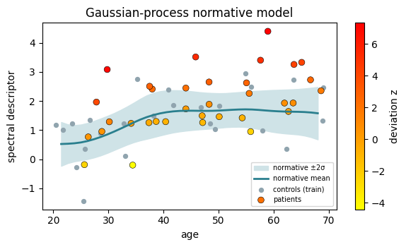
patient deviation z-scores: mean=1.39, 13 of 34 beyond z=+2
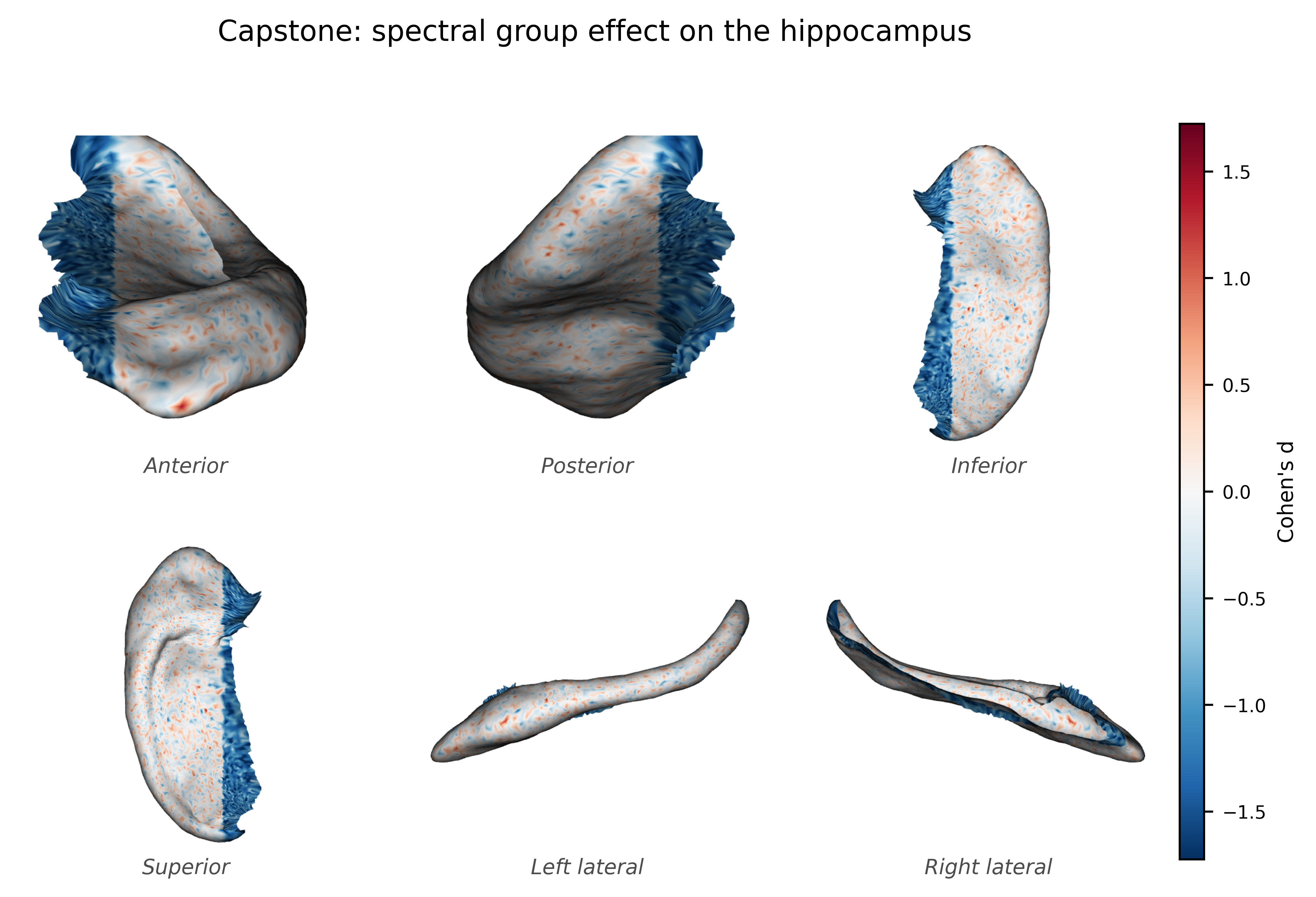
4. Capstone: back to the anatomy#
Every number above ultimately describes a brain structure. We close the loop by computing a per-vertex effect on the real left hippocampus and rendering it with the six-view tool, the same figure you would publish for a hippocampal sclerosis finding. (The two-group field is synthetic, planted in the head, as in notebook 8.)
from spectralbrain.viz import plot_surface_sixview
mesh = sb.BrainMesh(*sb.load_gifti_surface(
    data_path("hippunfold", "sub03", "hemi-L_space-T1w_den-8k_label-hipp_midthickness.surf.gii")))
dec = mesh.decompose(k=200)
field = np.asarray(sb.compute_hks(dec, n_times=100))[:, 60]
field = (field - field.mean()) / field.std()
head = mesh.vertices[:, 0] > np.percentile(mesh.vertices[:, 0], 80)

A = field[None, :] + rng.normal(0, 1, (16, mesh.n_vertices))
B = field[None, :] + rng.normal(0, 1, (16, mesh.n_vertices)); B[:, head] += 1.2
d_map = np.asarray(st.cohens_d_map(A, B))

fig = plot_surface_sixview(mesh, scalars=d_map, cmap="RdBu_r", signed=True,
                           scalar_bar_title="Cohen's d",
                           title="Capstone: spectral group effect on the hippocampus")
plt.show()
[06/09/26 02:34:19] INFO Laplacian (cotangent): N=8192, nnz=56578
2026-06-09 02:34:23.682 ( 1.059s) [ 7F8BD522C080]vtkXOpenGLRenderWindow.:1460 WARN| bad X server connection. DISPLAY=
The whole pipeline, in one breath#
You have now traversed the entire library:
LBO → the spectrum of a surface (notebook 1)
I/O → any neuroimaging format becomes a mesh or point cloud (2)
ShapeDNA → a global, pose-free fingerprint (3)
HKS / SI-HKS → local, multi-scale, scale-invariant descriptors (4)
WKS / GPS → band-pass descriptors and an embedding (5)
Point clouds & tracts → geometry without faces (6)
Functional maps & distances → relating shapes (7)
Cohorts & vertex-wise stats → where shapes differ, with FWE/FDR/TFCE (8)
Effect sizes & harmonisation → how much, how reliably, across sites (9)
Bayesian & visualization → uncertainty, sparsity, normative scores, figures (10)
From a triangle mesh to a posterior-backed, publication-ready anatomical map.
Exercises#
Sparsity vs signal. Add a third true predictor with a small coefficient (e.g. 0.3) and refit the horseshoe. Does it survive shrinkage? Tune
tau_prior.ROPE width. Re-run BEST with
rope=(-0.3, 0.3). How does the practical decision change for the same data?Kernel choice. Refit the normative model with
kernel='rbf'and'matern32'. How does the uncertainty band change, especially at the age extremes?Real outcome. Replace the synthetic outcome with a real per-subject summary (e.g. each subject’s mean HKS over vertices) from the four hippocampi and run the horseshoe on whatever covariate you have.
Posterior plots. Explore
spectralbrain.viz.bayes(plot_forest,plot_posterior) and reproduce the figures in sections 1–2 with the library’s own plotting helpers.
Where to go from here#
This series used five subjects to keep everything runnable; the same code scales
to full cohorts by swapping the loaders in notebook 2 for discover_bids /
discover_freesurfer and letting load_group stream subjects in parallel. The
methods transfer unchanged from the hippocampus to thalamic nuclei, cortical
surfaces, and white-matter tracts.
If you use SpectralBrain in your work, please cite the software (see the
repository CITATION.cff). Bug reports and contributions are welcome. Thank you
for working through the series.