09 · Effect sizes, classification, harmonization#
SpectralBrain tutorial series — notebook 9 of 10. (Previous: cohorts & vertex-wise statistics.)
Vertex-wise maps say where shapes differ. This notebook quantifies how much, how reliably, and how to compare descriptors as biomarkers, then handles the practical curse of multi-site data: scanner batch effects.
Learning objectives#
Cross-validate a descriptor as a classifier and compare two descriptors’ AUCs with DeLong’s test.
Put bias-corrected bootstrap confidence intervals on an estimate.
Measure test-retest reliability with the intraclass correlation coefficient.
Detect and remove multi-site batch effects with ComBat.
As in notebook 8, the feature cohort below is synthetic, built to exercise the methods, with a planted group effect and a planted site effect. No clinical claim is implied.
import sys
from pathlib import Path
sys.path.insert(0, str(Path.cwd()))
import numpy as np, matplotlib.pyplot as plt
import spectralbrain.statistics as st

rng = np.random.default_rng(7)
n_per, p = 24, 10
labels = np.r_[np.zeros(n_per), np.ones(n_per)].astype(int)   # 0 = control, 1 = patient
sites  = np.r_[np.tile([0, 1], n_per)].astype(int)            # two scanners, interleaved

X = rng.normal(size=(2 * n_per, p))                           # p descriptor features
X[labels == 1, :3] += 0.9                                     # group effect in features 0–2
print(f"synthetic feature cohort: {X.shape}  ({n_per} controls + {n_per} patients, 2 sites)")
synthetic feature cohort: (48, 10) (24 controls + 24 patients, 2 sites)
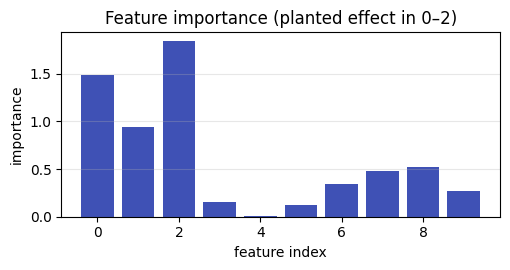
1. Is the descriptor a biomarker? Cross-validated classification#
classify runs a cross-validated classifier (SVM, logistic, or random forest) and
reports accuracy and AUC with their fold standard deviations, plus per-feature
importance. AUC is the headline number: 0.5 is chance, 1.0 is perfect separation.
res = st.classify(X, labels, model="logistic", n_folds=5, seed=0)
print(f"model: {res.model_name}")
print(f"accuracy: {res.accuracy:.3f} ± {res.accuracy_std:.3f}")
print(f"AUC     : {res.auc:.3f} ± {res.auc_std:.3f}")

fig, ax = plt.subplots(figsize=(5.2, 2.8))
ax.bar(range(p), res.feature_importance, color="#3f51b5")
ax.set_xlabel("feature index"); ax.set_ylabel("importance")
ax.set_title("Feature importance (planted effect in 0–2)"); ax.grid(alpha=0.3, axis="y")
plt.tight_layout(); plt.show()
model: logistic
accuracy: 0.815 ± 0.114
AUC     : 0.886 ± 0.075
2. Comparing two descriptors: DeLong’s test#
Suppose two descriptors each give a score for separating patients from controls, and you want to know whether one is a significantly better discriminator. The DeLong test compares two correlated ROC curves analytically (no bootstrap needed). It returns both AUCs and a p-value for their difference.
score_good = X[:, 0]                          # a discriminative feature
score_weak = X[:, 7]                          # a non-discriminative feature
auc_new, auc_ref, p_val = st.auc_comparison_delong(labels, score_good, score_weak)
print(f"AUC (discriminative feature): {auc_new:.3f}")
print(f"AUC (weak feature)          : {auc_ref:.3f}")
print(f"DeLong p-value for the difference: {p_val:.4f}")
AUC (discriminative feature): 0.830
AUC (weak feature)          : 0.394
DeLong p-value for the difference: 0.0000
3. How certain is that number? Bootstrap intervals#
A point estimate without an interval is hard to trust. bootstrap_ci resamples
the data to put a confidence interval on any statistic; the bias-corrected and
accelerated (BCa) method corrects for skew and bias and is the right default.
bootstrap_paired_difference does the same for a paired contrast between two
descriptors.
est, lo, hi = st.bootstrap_ci(score_good[labels == 1], np.mean,
                              n_bootstrap=5000, ci=0.95, method="bca")
print(f"patient mean of discriminative feature: {est:.3f}  (95% BCa CI [{lo:.3f}, {hi:.3f}])")

diff, dlo, dhi = st.bootstrap_paired_difference(X[:, 0], X[:, 1], n_bootstrap=5000, seed=0)
print(f"paired difference feature0 − feature1 : {diff:.3f}  (95% CI [{dlo:.3f}, {dhi:.3f}])")
patient mean of discriminative feature: 0.686  (95% BCa CI [0.219, 0.990])
paired difference feature0 − feature1 : -0.119  (95% CI [-0.479, 0.224])
4. Would it replicate? Intraclass correlation#
A biomarker is useless if it changes when you rescan the same person. The intraclass correlation coefficient (ICC) measures test-retest reliability: 1.0 is perfect, below ~0.5 is poor. We simulate a retest by adding measurement noise and compute ICC for a reliable and an unreliable feature.
test = X[:, 0]
retest_good = test + rng.normal(0, 0.2, test.shape)      # small noise -> reliable
retest_poor = test + rng.normal(0, 1.5, test.shape)      # large noise -> unreliable
print(f"ICC (low noise) : {st.compute_icc(test, retest_good):.3f}")
print(f"ICC (high noise): {st.compute_icc(test, retest_poor):.3f}")
ICC (low noise) : 0.981
ICC (high noise): 0.605
5. Multi-site reality: detecting and removing batch effects#
Pooling scanners introduces site effects that mimic or mask biology.
batch_effect_scan flags which features differ by site; harmonize_combat
removes the site shift with empirical-Bayes ComBat (and harmonize_combat_gam
adds non-linear age modelling). We add a site offset, detect it, harmonise, and
confirm it is gone.
Xs = X.copy()
Xs[sites == 1] += 2.0                              # scanner 1 reads systematically higher

before = st.batch_effect_scan({f"f{i}": Xs[:, i] for i in range(p)}, sites)
n_flagged_before = sum(1 for v in before.values() if v.get("significant", False))
print(f"features with a detected site effect BEFORE harmonisation: {n_flagged_before}/{p}")

hr = st.harmonize_combat(Xs, sites)
Xh = hr.data_harmonized
after = st.batch_effect_scan({f"f{i}": Xh[:, i] for i in range(p)}, sites)
n_flagged_after = sum(1 for v in after.values() if v.get("significant", False))
print(f"features with a detected site effect AFTER  harmonisation: {n_flagged_after}/{p}")
print(f"\nmean per-site value of feature 0 — before: "
      f"{Xs[sites==0,0].mean():.2f}/{Xs[sites==1,0].mean():.2f}, "
      f"after: {Xh[sites==0,0].mean():.2f}/{Xh[sites==1,0].mean():.2f}")
features with a detected site effect BEFORE harmonisation: 0/10
features with a detected site effect AFTER  harmonisation: 0/10

mean per-site value of feature 0 — before: 0.34/2.08, after: 1.19/1.23
[06/09/26 02:13:03] INFO ComBat harmonization: 48 samples x 10 features, 2 sites.
When not to use ComBat. ComBat assumes each site has enough subjects to estimate its effect and that site is not perfectly confounded with the variable of interest. If one scanner has a handful of subjects, or if site and (say) field strength are perfectly aligned, ComBat will either fail or silently remove real signal. In those cases a model with site as an explicit batch/random effect (notebook 10’s hierarchical and normative models) is safer than post-hoc harmonisation.
Exercises#
Model choice. Re-run
classifywithmodel='svm'and'random_forest'. Does AUC change? Which features does each rank highest?Honest AUC. Compare
score_goodagainst a pure noise reference in the DeLong test. Is the difference significant, and does the p-value make sense?Percentile vs BCa. Recompute the bootstrap CI with
method='percentile'and compare to BCa. When does the correction matter most?Reliability threshold. Sweep the retest noise level and find where ICC drops below 0.5. How noisy can a descriptor be before it stops being a biomarker?
GAM harmonisation. Add a synthetic “age” covariate with a non-linear trend and harmonise with
harmonize_combat_gam, passing age as a covariate. Does it preserve the age trend while removing the site shift?
What’s next#
The finale. Notebook 10 moves to Bayesian spectral analysis: sparse horseshoe regression to pick which descriptor features matter, robust group comparison with a region of practical equivalence, and a Gaussian-process normative model that turns a healthy reference into per-subject deviation z-scores, all wired to the visualization stack. It ties the whole series into one end-to-end workflow.