04 · The Heat Kernel Signature: diffusion as a local probe

SpectralBrain tutorial series — notebook 4 of 10. (Previous: ShapeDNA.)

ShapeDNA gave one fingerprint for a whole structure. To find out where shapes differ we need a descriptor at every vertex. The Heat Kernel Signature (HKS; Sun, Ovsjanikov & Guibas 2009) does exactly that, by watching how heat diffuses away from each point across many time scales.

Learning objectives

1. Define the HKS from the heat equation and the LBO spectrum.

2. See how scale (\(t\)) interpolates from local curvature to global shape.

3. Render HKS on the hippocampus and relate small-\(t\) HKS to curvature.

4. Make it scale-invariant with SI-HKS and prove the invariance.

1. Heat flow and the heat kernel

Drop a unit of heat at a point \(x\) and let it diffuse over the surface according to the heat equation \(\partial_t u = \Delta u\). The amount of heat remaining at \(x\) after time \(t\) — the heat kernel evaluated on the diagonal — has a clean spectral form:

\[\mathrm{HKS}(x, t) \;=\; k_t(x, x) \;=\; \sum_{k\ge 0} e^{-\lambda_k t}\,\varphi_k(x)^2 .\]

Read it as a recipe: each eigenfunction contributes its squared value, damped by \(e^{-\lambda_k t}\). The time \(t\) is a scale knob:

• small \(t\) — only the highest frequencies have not yet decayed, so HKS senses the immediate neighbourhood: curvature and fine geometry.

• large \(t\) — only the lowest frequencies survive, so HKS reflects the point’s place in the global shape.

Because it is built from \(\lambda_k\) and \(\varphi_k\), HKS inherits the LBO’s isometry invariance: it is intrinsic and pose-free, just like ShapeDNA, but resolved per vertex.

import sys
from pathlib import Path
sys.path.insert(0, str(Path.cwd()))
import numpy as np, matplotlib.pyplot as plt
import spectralbrain as sb
from _tutorial_utils import data_path

v, f = sb.load_gifti_surface(
    data_path("hippunfold", "sub03", "hemi-L_space-T1w_den-8k_label-hipp_midthickness.surf.gii"))
hipp = sb.BrainMesh(v, f)
dec = hipp.decompose(k=200)          # HKS wants more modes than ShapeDNA

# Principled time scales from the spectrum: t in [4 ln10 / λ_max , 4 ln10 / λ_1].
lam = dec.eigenvalues
t_min = 4 * np.log(10) / lam[-1]
t_max = 4 * np.log(10) / lam[1]
t_grid = np.logspace(np.log10(t_min), np.log10(t_max), 100)
hks = np.asarray(sb.compute_hks(dec, t_values=t_grid))
print(f"HKS matrix: {hks.shape}  (vertices x time-scales)")
print(f"time range: {t_min:.3g} ... {t_max:.3g}")

[06/09/26 02:00:22] INFO     Laplacian (cotangent): N=8192, nnz=56578                                              

HKS matrix: (8192, 100)  (vertices x time-scales)
time range: 3.54 ... 1.58e+03

2. One signature, many scales

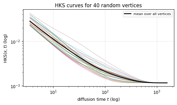
For a handful of vertices, plot HKS as a function of \(t\). Every curve is that point’s multi-scale identity card. Points in geometrically distinct locations (a tip vs a flat flank) trace different curves; the spread across vertices is largest at small \(t\) (local detail) and collapses at large \(t\) (everyone shares the same global shape).

rng = np.random.default_rng(0)
sample = rng.choice(hipp.n_vertices, 40, replace=False)
fig, ax = plt.subplots(figsize=(6, 3.6))
for idx in sample:
    ax.plot(t_grid, hks[idx], lw=0.7, alpha=0.5)
ax.plot(t_grid, hks.mean(0), "k-", lw=2, label="mean over all vertices")
ax.set_xscale("log"); ax.set_yscale("log")
ax.set_xlabel("diffusion time $t$ (log)"); ax.set_ylabel("HKS$(x,t)$ (log)")
ax.set_title("HKS curves for 40 random vertices"); ax.legend(fontsize=8); ax.grid(alpha=0.3)
plt.tight_layout(); plt.show()

3. The spatial pattern changes with scale

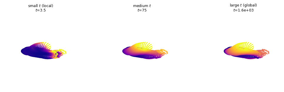
Now fix three scales — small, medium, large — and paint HKS across the surface. Watch the pattern reorganise: fine, curvature-driven structure at small \(t\) broadens into smooth, head-to-tail organisation at large \(t\).

t3 = np.logspace(np.log10(t_min), np.log10(t_max), 3)
hks3 = np.asarray(sb.compute_hks(dec, t_values=t3))

V = hipp.vertices
fig = plt.figure(figsize=(10.5, 3.2))
for i, (t, lab) in enumerate(zip(t3, ["small $t$ (local)", "medium $t$", "large $t$ (global)"])):
    ax = fig.add_subplot(1, 3, i + 1, projection="3d")
    s = hks3[:, i]
    ax.scatter(V[:, 0], V[:, 1], V[:, 2], c=s, cmap="plasma", s=2,
               vmin=np.percentile(s, 2), vmax=np.percentile(s, 98))
    ax.set_title(f"{lab}\n$t$={t:.2g}", fontsize=9); ax.set_axis_off(); ax.view_init(20, -70)
plt.tight_layout(); plt.show()

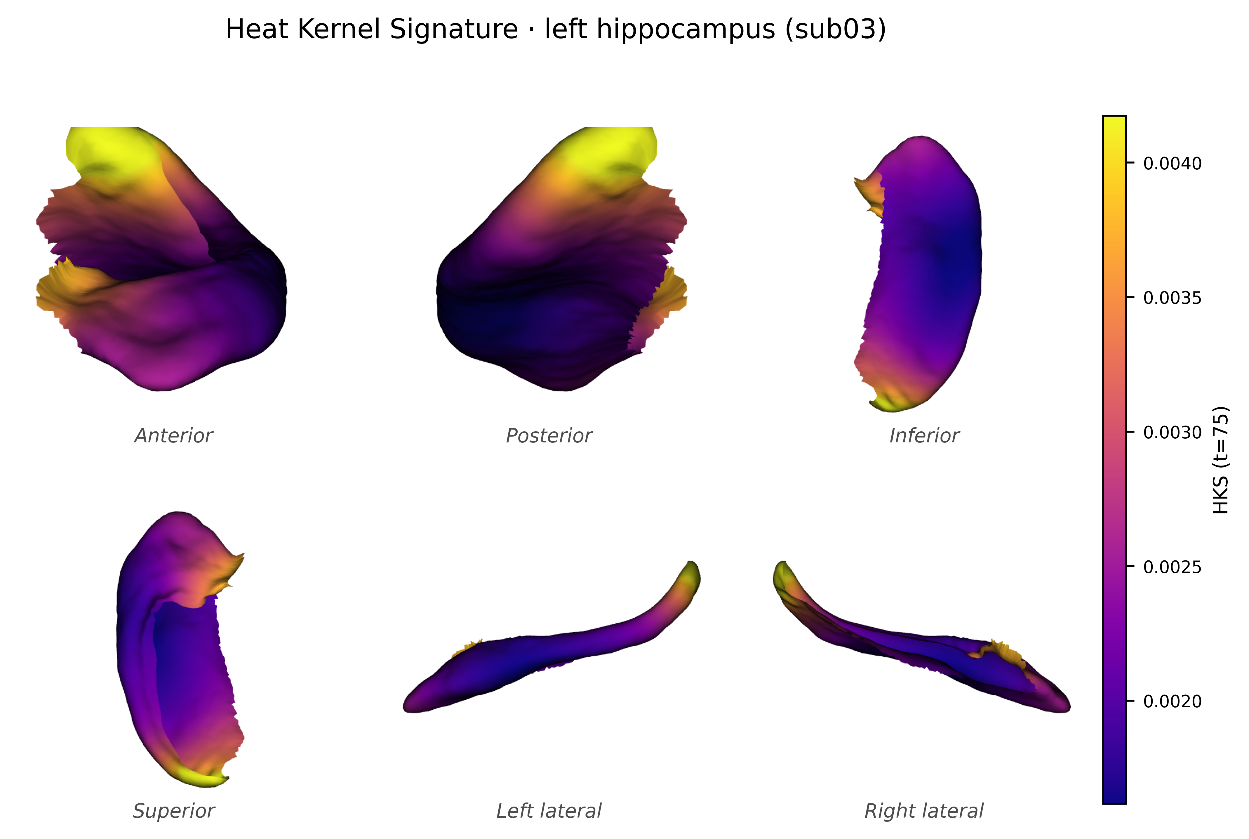
The same medium-scale HKS, rendered with the six-view tool — the kind of figure that goes into a paper.

from spectralbrain.viz import plot_surface_sixview
fig = plot_surface_sixview(hipp, scalars=hks3[:, 1], cmap="plasma",
                           scalar_bar_title=f"HKS (t={t3[1]:.2g})",
                           title="Heat Kernel Signature · left hippocampus (sub03)")
plt.show()

2026-06-09 02:00:28.159 (   0.510s) [    7F8673792080]vtkXOpenGLRenderWindow.:1460  WARN| bad X server connection. DISPLAY=

4. Small-\(t\) HKS is a curvature probe

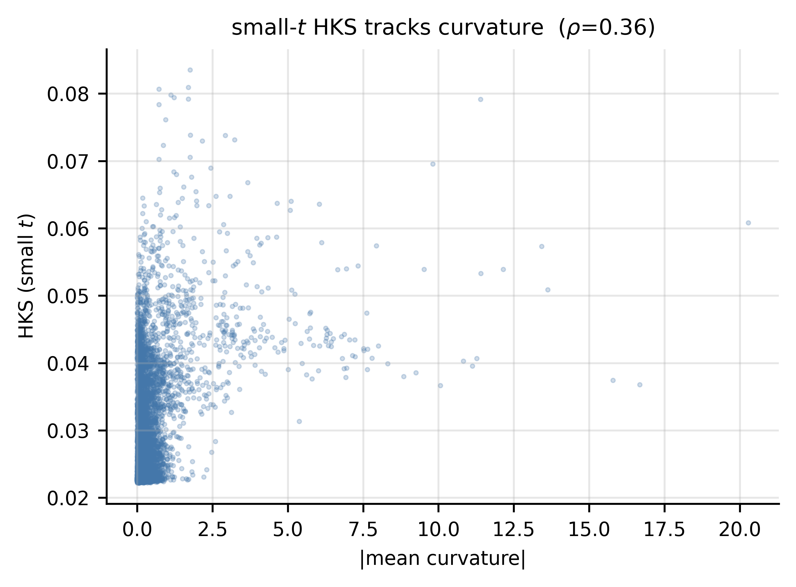
The short-time expansion of the heat kernel gives, to leading order,

\[\mathrm{HKS}(x, t) \;\approx\; \frac{1}{4\pi t}\Big(1 + \tfrac{t}{6}\,S(x) + \cdots\Big),\]

where \(S(x)\) is the scalar curvature (twice the Gaussian curvature on a surface). So at small \(t\), HKS should track curvature. We test it: correlate the smallest-\(t\) HKS column with the mesh’s own curvature estimate.

from scipy.stats import spearmanr
kmean = np.abs(hipp.mean_curvature())
rho, p = spearmanr(hks3[:, 0], kmean)
print(f"Spearman correlation (small-t HKS vs |mean curvature|): rho = {rho:.3f}, p = {p:.1e}")

fig, ax = plt.subplots(figsize=(4.6, 3.4))
ax.scatter(kmean, hks3[:, 0], s=3, alpha=0.25)
ax.set_xlabel("|mean curvature|"); ax.set_ylabel("HKS (small $t$)")
ax.set_title(f"small-$t$ HKS tracks curvature  ($\\rho$={rho:.2f})"); ax.grid(alpha=0.3)
plt.tight_layout(); plt.show()

Spearman correlation (small-t HKS vs |mean curvature|): rho = 0.355, p = 1.6e-242

5. The scale problem, and SI-HKS

HKS has one weakness for cross-subject work: it is not scale-invariant. Scaling a shape by \(\alpha\) rescales every eigenvalue by \(1/\alpha^2\), which slides the HKS curve along the \(t\)-axis. Two hippocampi of identical shape but different size get different HKS.

The Scale-Invariant HKS (Bronstein & Kokkinos 2010) fixes this with a neat trick: sample HKS on a logarithmic time grid (so a scale change becomes a shift), then take the magnitude of the Fourier transform along that axis (which is shift-invariant). compute_si_hks does this and returns a few low-frequency coefficients per vertex.

big = sb.BrainMesh(hipp.vertices * 2.0, hipp.faces)     # same shape, twice the size
dec_big = big.decompose(k=200)

# Plain HKS at fixed t: shifts with scale.
hks_o = np.asarray(sb.compute_hks(dec,     t_values=t3))
hks_b = np.asarray(sb.compute_hks(dec_big, t_values=t3))
print("plain HKS, mean value per scale:")
print(f"  original : {hks_o.mean(0)}")
print(f"  scaled x2: {hks_b.mean(0)}   <- different")

# SI-HKS: stable across scale (vertex order is preserved, so compare per-vertex).
si_o = np.asarray(sb.compute_si_hks(dec))
si_b = np.asarray(sb.compute_si_hks(dec_big))
corr = [np.corrcoef(si_o[:, j], si_b[:, j])[0, 1] for j in range(si_o.shape[1])]
print(f"\nSI-HKS per-frequency correlation (original vs scaled): "
      f"min={min(corr):.3f}, mean={np.mean(corr):.3f}")
print("-> SI-HKS is (nearly) invariant to the 2x rescaling; plain HKS is not.")

[06/09/26 02:00:32] INFO     Laplacian (cotangent): N=8192, nnz=56578                                              

plain HKS, mean value per scale:
  original : [0.02813216 0.00244451 0.00115613]
  scaled x2: [0.02352424 0.00166222 0.00032007]   <- different

SI-HKS per-frequency correlation (original vs scaled): min=1.000, mean=1.000
-> SI-HKS is (nearly) invariant to the 2x rescaling; plain HKS is not.

Exercises

1. Scale sweep. Plot mean HKS vs \(t\) for the original and the \(2\times\) mesh on the same log axes. Confirm the curve shifts horizontally by the predicted amount (\(\Delta\log t = \log \alpha^2\)).

2. Mode budget. Recompute HKS with k=50, 100, 200 modes. At which scale (\(t\)) does the number of modes matter most — small or large \(t\)? Why?

3. Curvature, properly. Replace mean_curvature with gaussian_curvature in section 4. Which curvature does small-\(t\) HKS track more tightly, and does the short-time expansion explain it?

4. Subfield contrast. Render HKS at small \(t\) on the hippocampal tail surface from notebook 2 and compare its curvature structure to the full hippocampus.

5. Descriptor as feature. Take the full HKS matrix (100 scales) for sub03_L and sub04_L, average over vertices, and measure the Euclidean distance between the two mean-HKS curves. How does it compare to their ShapeDNA distance from notebook 3?

What’s next

HKS is a low-pass descriptor: heat diffusion smooths away high frequencies. Notebook 05 introduces the Wave Kernel Signature, which uses the Schrödinger equation to build a band-pass descriptor with sharper frequency localisation, plus the Global Point Signature embedding. Together they round out the per-vertex descriptor toolkit before we turn to correspondence and statistics.