06 · Point clouds & white-matter tracts#
SpectralBrain tutorial series — notebook 6 of 10. (Previous: WKS & GPS.)
Every structure so far was a closed surface mesh. White-matter bundles are different: a TractSeg segmentation is a cloud of voxels with no natural surface and no faces. This notebook handles geometry without connectivity, using the robust (intrinsic) Laplacian, and introduces the point-cloud spectral signatures, with the numerical cautions they demand.
Learning objectives#
Build an LBO on a point cloud with no faces (the robust Laplacian).
Compute HKS / WKS on white-matter bundles from subject 05.
Use the point-cloud signatures BKS / iBKS, and respect their numerical limits.
Compare bundles by their spectra.
1. A Laplacian without faces#
The cotangent Laplacian of notebook 1 needs triangles: it sums cotangents of
triangle angles. A point cloud has none. The robust Laplacian (Sharp & Crane
2020) solves this by building a local “tufted” triangulation around each point and
defining a Laplace operator on that intrinsic structure. The upshot: any
\(N\times 3\) array of points gets a spectrum, eigenfunctions, and therefore every
descriptor in this series, with no meshing step. SpectralBrain selects it
automatically for a BrainPointCloud.
Requires
pip install robust_laplacian.
import sys
from pathlib import Path
sys.path.insert(0, str(Path.cwd()))
import numpy as np, matplotlib.pyplot as plt
import spectralbrain as sb
from _tutorial_utils import data_path

clouds = sb.load_tractseg(data_path("tractseg", "sub05"), output="pointcloud")
print(f"{len(clouds)} white-matter bundles loaded as point clouds.")
for name in ["CA", "SCP_left", "ILF_left", "CST_left"]:
    print(f"  {name:10s}: {clouds[name].points.shape[0]:,} points")
[06/09/26 02:07:25] INFO     TractSeg: 15 bundle masks in
                             /home/claude/work/spectralbrain-main/tutorials/data/tractseg/sub05/bundle_segmentation
                             s
[06/09/26 02:07:25] INFO Extracted 47086 points for label 1
INFO Extracted 45527 points for label 1
INFO Extracted 3048 points for label 1
INFO Extracted 302867 points for label 1
INFO Extracted 20324 points for label 1
INFO Extracted 19332 points for label 1
INFO Extracted 46771 points for label 1
INFO Extracted 48325 points for label 1
INFO Extracted 17846 points for label 1
INFO Extracted 16753 points for label 1
INFO Extracted 32051 points for label 1
[06/09/26 02:07:26] INFO Extracted 52144 points for label 1
INFO Extracted 50127 points for label 1
INFO Extracted 13036 points for label 1
INFO Extracted 13591 points for label 1
[06/09/26 02:07:26] INFO Loaded 15/15 TractSeg bundles as pointcloud.
15 white-matter bundles loaded as point clouds.
  CA        : 3,048 points
  SCP_left  : 13,036 points
  ILF_left  : 17,846 points
  CST_left  : 20,324 points
2. Descriptors on a bundle#
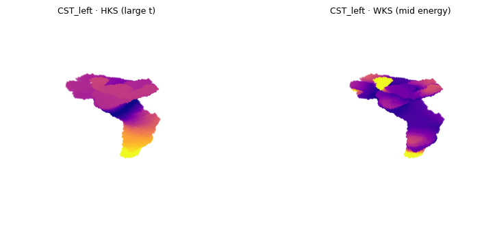
We take the left corticospinal tract (CST), decompose it, and compute HKS and WKS exactly as for a mesh. The descriptors flow along the bundle, picking out its elongated geometry.
cst = clouds["CST_left"]
dec = cst.decompose(k=60)
hks = np.asarray(sb.compute_hks(dec, n_times=100))
wks = np.asarray(sb.compute_wks(dec, n_energies=100))
print(f"CST_left: {cst.points.shape[0]:,} points -> lambda_1={dec.eigenvalues[1]:.3e}")

P = cst.points
fig = plt.figure(figsize=(9, 3.4))
for i, (desc, t, ttl) in enumerate([(hks, 60, "HKS (large t)"), (wks, 50, "WKS (mid energy)")]):
    ax = fig.add_subplot(1, 2, i + 1, projection="3d")
    s = desc[:, t]
    ax.scatter(P[:, 0], P[:, 1], P[:, 2], c=s, cmap="plasma", s=2,
               vmin=np.percentile(s, 2), vmax=np.percentile(s, 98))
    ax.set_title(f"CST_left · {ttl}", fontsize=9); ax.set_axis_off(); ax.view_init(15, -75)
plt.tight_layout(); plt.show()
[06/09/26 02:07:26] INFO Point cloud Laplacian (robust): N=20324, nnz=229438
CST_left: 20,324 points -> lambda_1=2.295e-04
3. Point-cloud spectral signatures: BKS and iBKS#
Bates et al. (2011) introduced spectral signatures tailored to point clouds for
neuroimaging. SpectralBrain provides the BKS (compute_bks), its improved
curvature-aware variant iBKS (compute_ibks), and the multi-time Bates
signatures (compute_bates_signatures).
A genuine caution. BKS can be numerically explosive: on poorly conditioned clouds its values have been observed to reach \(10^{30}\) and beyond, which wrecks any downstream statistic. Always inspect its range before using it, prefer iBKS (which is regularised), and exclude BKS if it blows up. We check the range here.
bks  = np.asarray(sb.compute_bks(dec))
ibks = np.asarray(sb.compute_ibks(dec))
bates = np.asarray(sb.compute_bates_signatures(dec, n_times=10))
print(f"BKS   range: {bks.min():.3e} .. {bks.max():.3e}")
print(f"iBKS  range: {ibks.min():.3e} .. {ibks.max():.3e}")
print(f"Bates signatures shape: {bates.shape}")
if bks.max() > 1e6 or not np.isfinite(bks).all():
    print("\n*** BKS is out of safe range here — exclude it from statistics. ***")
else:
    print("\nBKS is within a usable range for this bundle (still prefer iBKS for robustness).")
BKS   range: 3.059e+01 .. 1.248e+03
iBKS  range: 3.059e+01 .. 1.248e+03
Bates signatures shape: (20324, 20)

BKS is within a usable range for this bundle (still prefer iBKS for robustness).
4. Comparing bundles by their spectra#
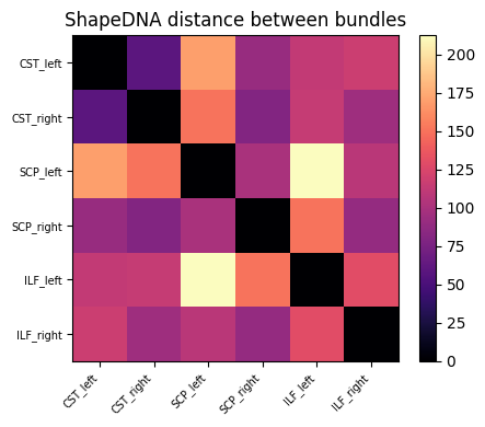
Because the spectrum is pose- and size-normalisable (notebook 3), we can compare different bundles by their ShapeDNA. We decompose a set of bilateral tracts and cluster them. Bundles that are geometrically alike (left/right of the same tract) should land near each other.
subset = ["CST_left", "CST_right", "SCP_left", "SCP_right", "ILF_left", "ILF_right"]
dnas = {}
for name in subset:
    d = clouds[name].decompose(k=40)
    dnas[name] = sb.compute_shapedna(d, normalize="area")
    print(f"  {name:11s} decomposed ({clouds[name].points.shape[0]:,} pts)")

D = np.zeros((len(subset), len(subset)))
for i, a in enumerate(subset):
    for j, b in enumerate(subset):
        D[i, j] = sb.shapedna_distance(dnas[a], dnas[b])

fig, ax = plt.subplots(figsize=(4.8, 4.0))
im = ax.imshow(D, cmap="magma")
ax.set_xticks(range(len(subset))); ax.set_yticks(range(len(subset)))
ax.set_xticklabels(subset, rotation=45, ha="right", fontsize=7); ax.set_yticklabels(subset, fontsize=7)
ax.set_title("ShapeDNA distance between bundles"); plt.colorbar(im, fraction=0.046)
plt.tight_layout(); plt.show()
  CST_left    decomposed (20,324 pts)
  CST_right   decomposed (19,332 pts)
  SCP_left    decomposed (13,036 pts)
  SCP_right   decomposed (13,591 pts)
  ILF_left    decomposed (17,846 pts)
  ILF_right   decomposed (16,753 pts)
[06/09/26 02:07:37] INFO Point cloud Laplacian (robust): N=19332, nnz=214356
[06/09/26 02:07:40] INFO Point cloud Laplacian (robust): N=13036, nnz=147996
[06/09/26 02:07:42] INFO Point cloud Laplacian (robust): N=13591, nnz=152465
[06/09/26 02:07:45] INFO Point cloud Laplacian (robust): N=17846, nnz=195718
[06/09/26 02:07:48] INFO Point cloud Laplacian (robust): N=16753, nnz=183537
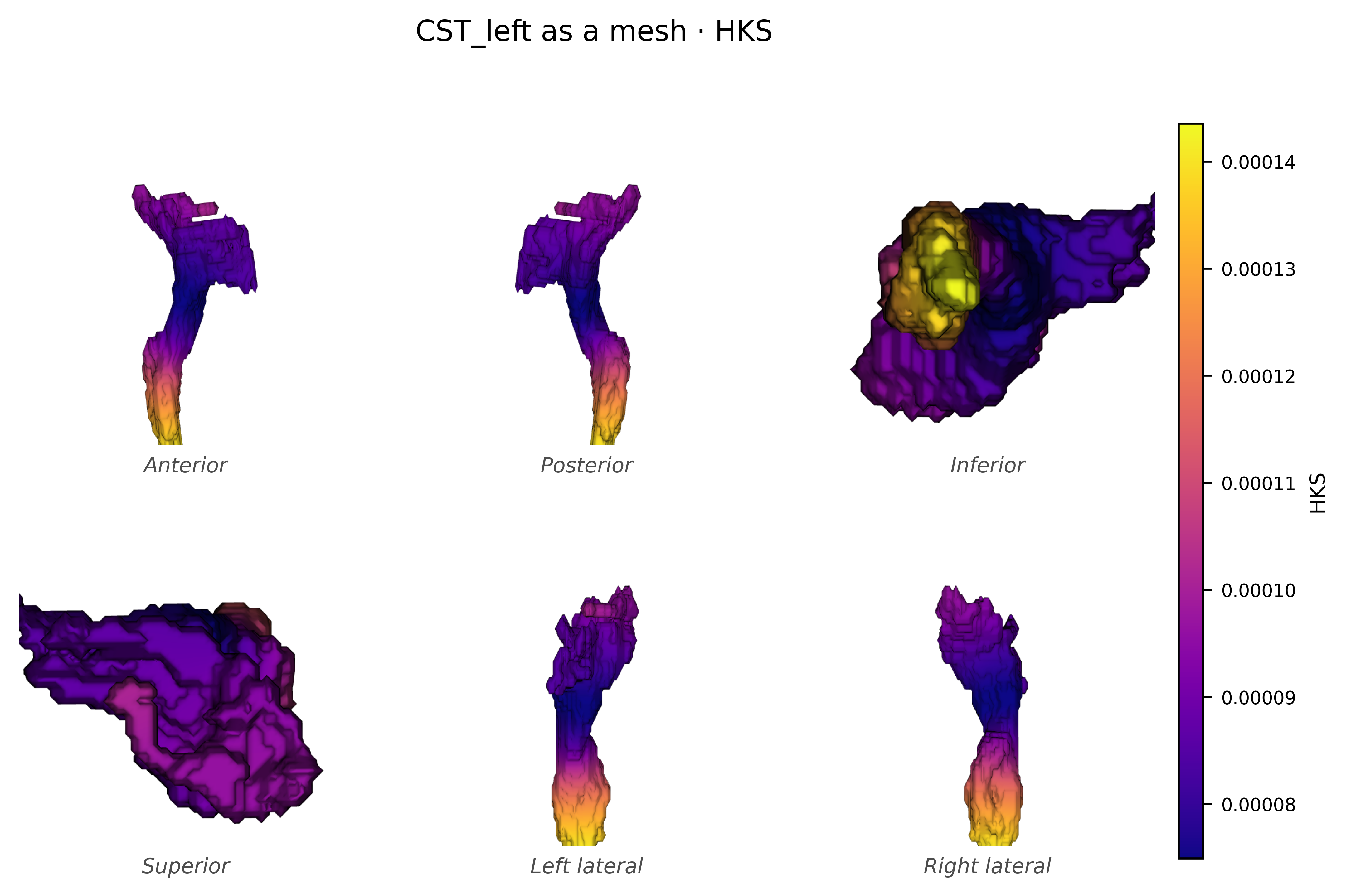
5. The same bundle, as a mesh#
For comparison, load CST as a marching-cubes mesh (cotangent Laplacian) and render its HKS with the six-view tool, the surface counterpart of the point-cloud scatter above.
from spectralbrain.viz import plot_surface_sixview
cst_mesh = sb.load_tractseg(data_path("tractseg", "sub05"), output="mesh")["CST_left"]
dm = cst_mesh.decompose(k=60)
hks_m = np.asarray(sb.compute_hks(dm, n_times=100))
fig = plot_surface_sixview(cst_mesh, scalars=hks_m[:, 60], cmap="plasma",
                           scalar_bar_title="HKS", title="CST_left as a mesh · HKS")
plt.show()
[06/09/26 02:07:51] INFO     TractSeg: 15 bundle masks in
                             /home/claude/work/spectralbrain-main/tutorials/data/tractseg/sub05/bundle_segmentation
                             s
[06/09/26 02:07:53] INFO Loaded 15/15 TractSeg bundles as mesh.
[06/09/26 02:07:53] INFO Laplacian (cotangent): N=11379, nnz=79677
2026-06-09 02:07:54.857 ( 0.282s) [ 7FAD82AD6080]vtkXOpenGLRenderWindow.:1460 WARN| bad X server connection. DISPLAY=
Exercises#
Resolution. The corpus callosum (
CC) has ~300k points. Decompose it withk=40and time it. Why is the robust Laplacian on a large cloud expensive, and what would you downsample to?iBKS vs BKS. Plot BKS and iBKS along the CST. Where do they disagree, and which looks more physically plausible (smooth along the bundle)?
Bilateral symmetry. From the distance matrix, is each tract closer to its contralateral twin than to other tracts? Quantify it.
Mesh vs cloud spectra. Overlay the first 40 eigenvalues of
CST_leftas a point cloud and as a mesh. Where do they diverge, and why might that be?A small bundle. Decompose the anterior commissure (
CA, ~3k points) and check whetherk=40is even well-defined for so few points.
What’s next#
We can now describe any surface or cloud. Notebook 07 asks how to relate two shapes: functional maps that transfer information between hippocampi, intrinsic distances within a shape (biharmonic, commute-time, diffusion), and point-set distances between shapes (Chamfer, Hausdorff).