05 · Wave Kernel Signature & Global Point Signature

SpectralBrain tutorial series — notebook 5 of 10. (Previous: the Heat Kernel Signature.)

HKS is a low-pass descriptor: heat diffusion erases high frequencies, so HKS emphasises coarse structure as \(t\) grows. Two complementary descriptors complete the per-vertex toolkit: the Wave Kernel Signature (WKS), a band-pass descriptor with sharp frequency localisation, and the Global Point Signature (GPS), an isometry-invariant embedding of the surface into a feature space.

Learning objectives

1. Define the WKS from the Schrödinger equation and contrast band-pass vs low-pass.

2. Compute and render WKS at several energies on the hippocampus.

3. Build the GPS embedding and understand its geometric meaning.

1. From heat to waves

HKS came from the heat equation \(\partial_t u = \Delta u\), whose solutions decay. The WKS (Aubry, Schlickewei & Cremers 2011) instead follows the Schrödinger equation \(\partial_t \psi = i\Delta\psi\), whose solutions oscillate. A quantum particle with an energy distribution centred at \(e\) has, at vertex \(x\), the probability

\[\mathrm{WKS}(x, e) \;\propto\; \sum_{k} e^{-\,(e - \log\lambda_k)^2 / 2\sigma^2}\;\varphi_k(x)^2 .\]

The Gaussian in \(\log\lambda\) acts as a band-pass filter: each energy \(e\) picks out a narrow band of eigenfrequencies. Compare this to HKS, whose \(e^{-\lambda t}\) weight is a low-pass filter that always includes everything below a cutoff. The practical consequence: WKS separates features that live at specific spatial frequencies, giving it crisper localisation, while HKS gives smoother, more stable maps. They are complementary, and SpectralBrain offers both.

import sys
from pathlib import Path
sys.path.insert(0, str(Path.cwd()))
import numpy as np, matplotlib.pyplot as plt
import spectralbrain as sb
from _tutorial_utils import data_path

v, f = sb.load_gifti_surface(
    data_path("hippunfold", "sub03", "hemi-L_space-T1w_den-8k_label-hipp_midthickness.surf.gii"))
hipp = sb.BrainMesh(v, f)
dec = hipp.decompose(k=200)

wks = np.asarray(sb.compute_wks(dec, n_energies=100))
print(f"WKS matrix: {wks.shape}  (vertices x energies)")

[06/09/26 02:06:15] INFO     Laplacian (cotangent): N=8192, nnz=56578                                              

WKS matrix: (8192, 100)  (vertices x energies)

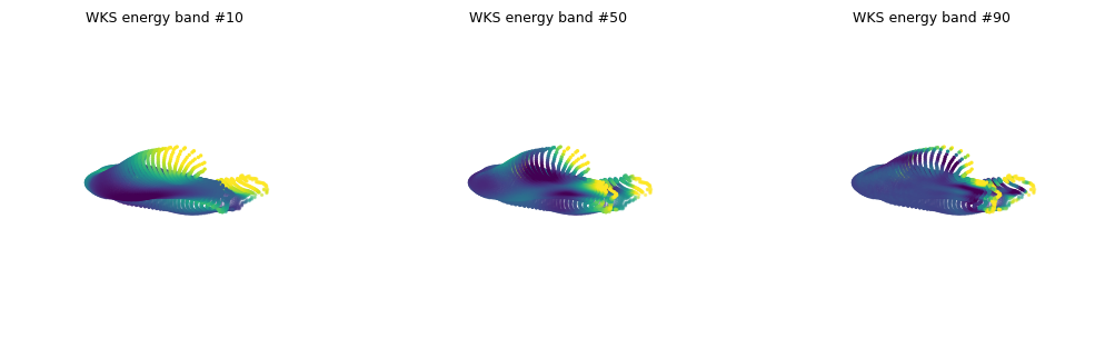
2. WKS across energies: band-pass in action

Each energy column highlights a different spatial frequency band. Low energy = coarse, high energy = fine. Painting three energies on the surface shows the band-pass behaviour: distinct, non-nested patterns, unlike HKS where larger \(t\) simply blurs smaller \(t\).

cols = [10, 50, 90]                       # low / mid / high energy bands
V = hipp.vertices
fig = plt.figure(figsize=(10.5, 3.2))
for i, c in enumerate(cols):
    ax = fig.add_subplot(1, 3, i + 1, projection="3d")
    s = wks[:, c]
    ax.scatter(V[:, 0], V[:, 1], V[:, 2], c=s, cmap="viridis", s=2,
               vmin=np.percentile(s, 2), vmax=np.percentile(s, 98))
    ax.set_title(f"WKS energy band #{c}", fontsize=9); ax.set_axis_off(); ax.view_init(20, -70)
plt.tight_layout(); plt.show()

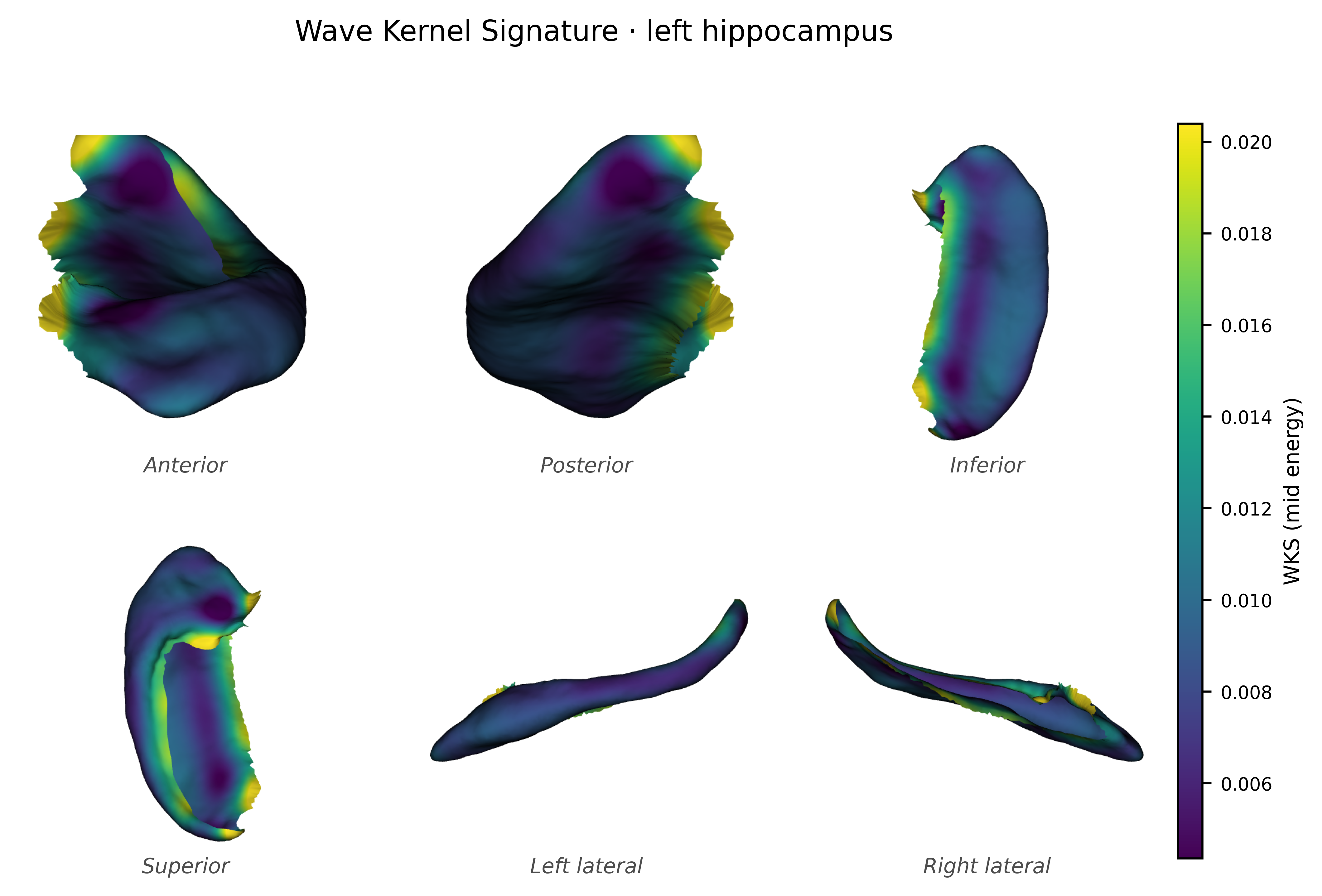
from spectralbrain.viz import plot_surface_sixview
fig = plot_surface_sixview(hipp, scalars=wks[:, 50], cmap="viridis",
                           scalar_bar_title="WKS (mid energy)",
                           title="Wave Kernel Signature · left hippocampus")
plt.show()

2026-06-09 02:06:19.717 (   0.280s) [    7FCAAF9AF080]vtkXOpenGLRenderWindow.:1460  WARN| bad X server connection. DISPLAY=

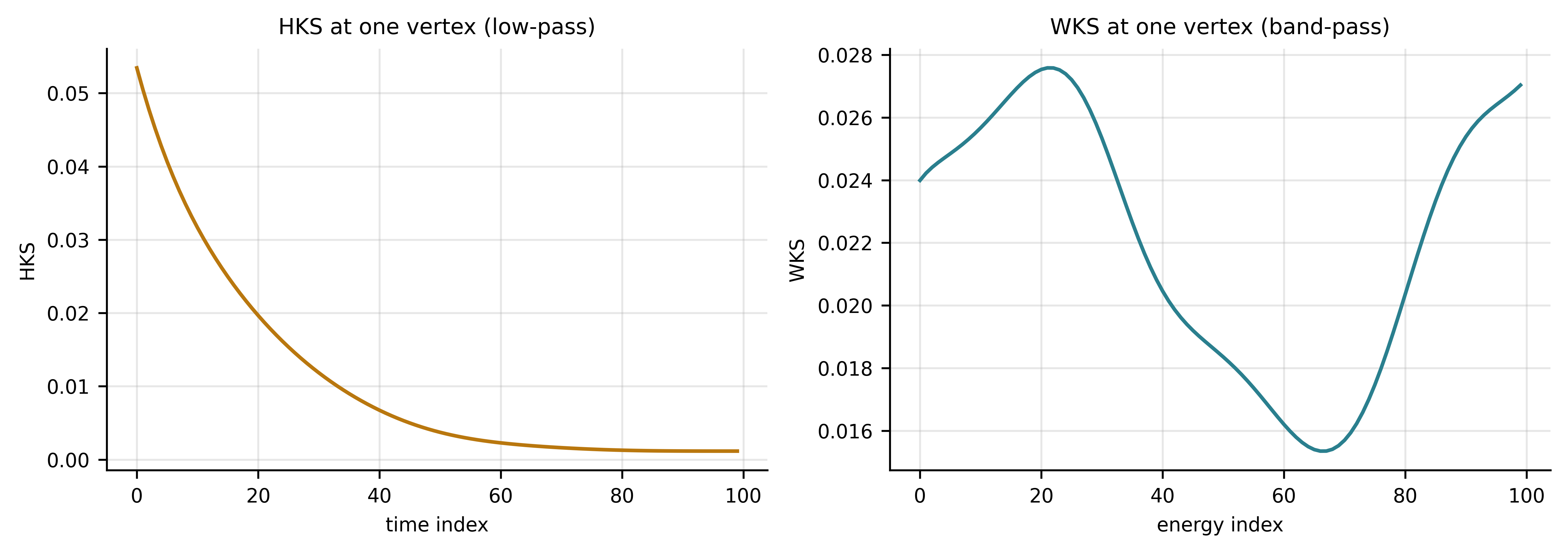
3. Low-pass vs band-pass, side by side

To make the filtering difference concrete, plot the HKS and WKS “response” at one vertex as a function of scale/energy. HKS falls monotonically (low-pass); WKS has a localised bump (band-pass).

hks = np.asarray(sb.compute_hks(dec, n_times=100))
idx = hipp.n_vertices // 2
fig, axes = plt.subplots(1, 2, figsize=(9, 3.2))
axes[0].plot(hks[idx], color="#b9770e"); axes[0].set_title("HKS at one vertex (low-pass)")
axes[0].set_xlabel("time index"); axes[0].set_ylabel("HKS")
axes[1].plot(wks[idx], color="#2a7f8e"); axes[1].set_title("WKS at one vertex (band-pass)")
axes[1].set_xlabel("energy index"); axes[1].set_ylabel("WKS")
for ax in axes: ax.grid(alpha=0.3)
plt.tight_layout(); plt.show()

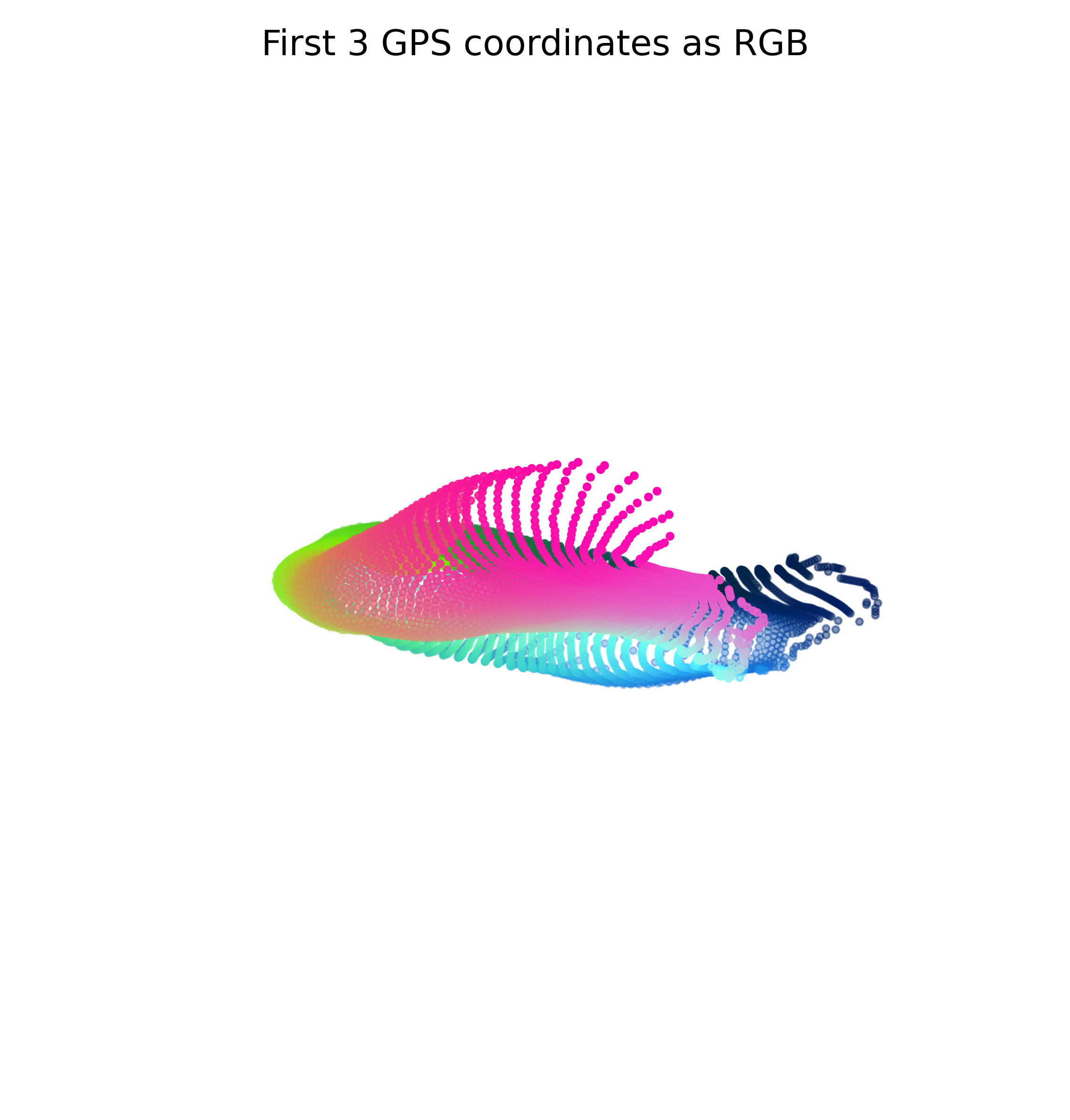
4. The Global Point Signature: shape as an embedding

GPS (Rustamov 2007) takes a different route. Instead of a multi-scale curve per vertex, it maps each vertex to a single point in an infinite-dimensional space:

\[\mathrm{GPS}(x) \;=\; \Big(\tfrac{\varphi_1(x)}{\sqrt{\lambda_1}},\, \tfrac{\varphi_2(x)}{\sqrt{\lambda_2}},\, \tfrac{\varphi_3(x)}{\sqrt{\lambda_3}},\, \dots \Big).\]

Two properties make this useful. The scaling by \(1/\sqrt{\lambda_k}\) damps high-frequency noise, and Euclidean distance in GPS space approximates an intrinsic distance on the surface (closely related to the biharmonic distance of notebook 7). So GPS turns “how far apart are two points along the shape” into an ordinary distance you can feed to clustering or correspondence.

gps = np.asarray(sb.compute_gps(dec))
print(f"GPS embedding: {gps.shape}  (vertices x coordinates)")

# Colour the surface by the first three GPS coordinates (an RGB-like shape code).
g3 = gps[:, :3]
g3 = (g3 - g3.min(0)) / (np.ptp(g3, axis=0) + 1e-12)
fig = plt.figure(figsize=(4.6, 4.0)); ax = fig.add_subplot(111, projection="3d")
ax.scatter(V[:, 0], V[:, 1], V[:, 2], c=g3, s=3)
ax.set_title("First 3 GPS coordinates as RGB"); ax.set_axis_off(); ax.view_init(20, -70)
plt.tight_layout(); plt.show()

GPS embedding: (8192, 199)  (vertices x coordinates)

Exercises

1. Energy budget. Recompute WKS with n_energies=50 and 200. Does the localisation of band #50 change? Relate this to the sigma parameter.

2. HKS vs WKS discrimination. For sub03_L and sub04_L, average each descriptor over vertices and measure the distance between subjects with HKS vs with WKS. Which separates them more?

3. GPS distance. Pick two vertices on opposite ends of the hippocampus and compute their Euclidean distance in GPS space; compare to a near pair. Does GPS distance grow with geodesic separation?

4. Noise damping. Plot the magnitude of GPS coordinates vs index. Confirm the \(1/\sqrt{\lambda_k}\) weighting suppresses high-index (noisy) modes.

5. WKS on a tract. Foreshadow notebook 6: load a TractSeg bundle as a point cloud and compute its WKS. Does band-pass structure appear along the bundle?

What’s next

So far every structure was a closed surface mesh. Notebook 06 turns to point clouds and white-matter tracts: the robust Laplacian that needs no faces, the point-cloud spectral signatures (BKS / iBKS), and the numerical cautions that come with them.