03 · ShapeDNA: hearing the shape of a hippocampus#
SpectralBrain tutorial series — notebook 3 of 10. (Previous: the I/O layer.)
Notebook 1 ended on a cliff-hanger: rigid motion leaves the spectrum unchanged, so the eigenvalues themselves are a pose-free fingerprint of shape. That fingerprint is ShapeDNA (Reuter, Wolter & Peinecke 2006). Here we compute it on the four HippUnfold hippocampi from notebook 2 and use it to quantify left–right asymmetry and between-subject differences — without ever aligning the shapes.
Learning objectives#
Explain why the eigenvalue sequence encodes geometry (heat-trace asymptotics).
Compute ShapeDNA with
compute_shapednaand read its normalization options.Make ShapeDNA scale-invariant and measure shape distance between structures.
1. What the spectrum knows#
ShapeDNA is just the truncated, ordered eigenvalue sequence \((\lambda_1, \lambda_2, \dots, \lambda_k)\) (we skip \(\lambda_0 = 0\)). Why should a list of numbers describe a shape? The heat-trace asymptotic expansion answers this. The sum \(\sum_k e^{-\lambda_k t}\) behaves, for small diffusion time \(t\), as
where \(A\) is the surface area, \(L\) the boundary length, and \(\int K\,dA\) the integrated Gaussian curvature (a topological constant by Gauss–Bonnet). So the eigenvalues collectively carry area, perimeter, and curvature — the geometry of the structure. Weyl’s law (notebook 1) is the leading term. ShapeDNA packs this information into a short, comparable vector.
import sys
from pathlib import Path
sys.path.insert(0, str(Path.cwd()))
import numpy as np, matplotlib.pyplot as plt
import spectralbrain as sb
from _tutorial_utils import data_path, spectrum_plot

# Load the four HippUnfold hippocampi (sub03/sub04, left/right) from notebook 2.
hipp = {}
for sid in ["sub03", "sub04"]:
    for hemi in ["L", "R"]:
        p = data_path("hippunfold", sid, f"hemi-{hemi}_space-T1w_den-8k_label-hipp_midthickness.surf.gii")
        v, f = sb.load_gifti_surface(p)
        hipp[f"{sid}_{hemi}"] = sb.BrainMesh(v, f)

decs = {name: m.decompose(k=80) for name, m in hipp.items()}
print("decomposed:", ", ".join(decs))
[06/09/26 01:58:40] INFO Laplacian (cotangent): N=8192, nnz=56578
[06/09/26 01:58:41] INFO Laplacian (cotangent): N=8192, nnz=56578
[06/09/26 01:58:42] INFO Laplacian (cotangent): N=8192, nnz=56578
[06/09/26 01:58:43] INFO Laplacian (cotangent): N=8192, nnz=56578
decomposed: sub03_L, sub03_R, sub04_L, sub04_R
2. Computing ShapeDNA#
compute_shapedna(dec, normalize=...) returns the descriptor. The normalize
argument is the important choice:
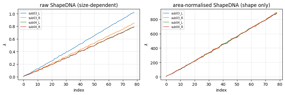
normalize='none'— raw eigenvalues. These depend on size: a bigger hippocampus has smaller eigenvalues (recall \(\lambda \propto 1/\text{area}\)).normalize='area'(default) — scales out the surface area, so ShapeDNA reflects shape, not size. Use this to compare structures of different sizes.
dna_raw  = {n: np.asarray(sb.compute_shapedna(d, normalize="none")) for n, d in decs.items()}
dna_norm = {n: np.asarray(sb.compute_shapedna(d, normalize="area")) for n, d in decs.items()}

fig, axes = plt.subplots(1, 2, figsize=(10, 3.4))
for n in decs:
    axes[0].plot(dna_raw[n], lw=1, label=n)
    axes[1].plot(dna_norm[n], lw=1, label=n)
axes[0].set_title("raw ShapeDNA (size-dependent)")
axes[1].set_title("area-normalised ShapeDNA (shape only)")
for ax in axes:
    ax.set_xlabel("index"); ax.set_ylabel(r"$\lambda$"); ax.grid(alpha=0.3); ax.legend(fontsize=7)
plt.tight_layout(); plt.show()
3. Scale invariance, demonstrated#
If ShapeDNA truly describes shape, scaling a hippocampus should leave the
normalised descriptor unchanged while the raw one shifts. We scale sub03_L
by a factor of 2 (its area grows \(4\times\), so raw eigenvalues shrink \(4\times\))
and check both descriptors.
big = sb.BrainMesh(hipp["sub03_L"].vertices * 2.0, hipp["sub03_L"].faces)
dec_big = big.decompose(k=80)

raw_ratio  = np.asarray(sb.compute_shapedna(dec_big, normalize="none")) / dna_raw["sub03_L"]
norm_diff  = np.abs(np.asarray(sb.compute_shapedna(dec_big, normalize="area")) - dna_norm["sub03_L"])
print(f"raw eigenvalue ratio (scaled / original): mean = {raw_ratio.mean():.3f}  (expected 0.25)")
print(f"normalised ShapeDNA: max |difference| = {norm_diff.max():.3e}  (expected ~0)")
print("\n-> raw ShapeDNA tracks size; area-normalised ShapeDNA is scale-invariant.")
[06/09/26 01:58:45] INFO Laplacian (cotangent): N=8192, nnz=56578
raw eigenvalue ratio (scaled / original): mean = 0.250  (expected 0.25)
normalised ShapeDNA: max |difference| = 2.387e-12  (expected ~0)

-> raw ShapeDNA tracks size; area-normalised ShapeDNA is scale-invariant.
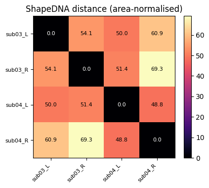
4. Comparing shapes: ShapeDNA distance#
shapedna_distance(a, b, metric=...) reduces two fingerprints to a single number.
With area-normalised descriptors it measures pure shape dissimilarity. We build
the full \(4\times4\) distance matrix over the hippocampi.
names = list(decs)
dnas = {n: sb.compute_shapedna(decs[n], normalize="area") for n in names}
D = np.zeros((4, 4))
for i, a in enumerate(names):
    for j, b in enumerate(names):
        D[i, j] = sb.shapedna_distance(dnas[a], dnas[b], metric="euclidean")

fig, ax = plt.subplots(figsize=(4.6, 3.9))
im = ax.imshow(D, cmap="magma")
ax.set_xticks(range(4)); ax.set_yticks(range(4))
ax.set_xticklabels(names, rotation=45, ha="right", fontsize=8); ax.set_yticklabels(names, fontsize=8)
for i in range(4):
    for j in range(4):
        ax.text(j, i, f"{D[i, j]:.1f}", ha="center", va="center",
                color="white" if D[i, j] < D.max() * 0.6 else "black", fontsize=8)
ax.set_title("ShapeDNA distance (area-normalised)")
plt.colorbar(im, fraction=0.046); plt.tight_layout(); plt.show()
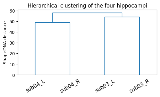
5. Reading the matrix: asymmetry and clustering#
Two questions the matrix answers at a glance: how different are a subject’s left and right hippocampi (asymmetry), and do subjects separate? A dendrogram on the same distances makes the grouping explicit.
# Left-right asymmetry per subject = distance between that subject's L and R.
for sid in ["sub03", "sub04"]:
    i, j = names.index(f"{sid}_L"), names.index(f"{sid}_R")
    print(f"{sid} left–right ShapeDNA asymmetry: {D[i, j]:.2f}")

from scipy.cluster.hierarchy import linkage, dendrogram
from scipy.spatial.distance import squareform
Z = linkage(squareform(D, checks=False), method="average")
fig, ax = plt.subplots(figsize=(5.2, 3.2))
dendrogram(Z, labels=names, ax=ax, leaf_rotation=30)
ax.set_ylabel("ShapeDNA distance"); ax.set_title("Hierarchical clustering of the four hippocampi")
plt.tight_layout(); plt.show()
sub03 left–right ShapeDNA asymmetry: 54.12

sub04 left–right ShapeDNA asymmetry: 48.83
6. What ShapeDNA cannot do#
ShapeDNA is global: it summarises the whole structure in one vector. That is
its strength (compact, pose-free, fast) and its limit — it cannot tell you where
two shapes differ. A focal change in the hippocampal head and the same-magnitude
change in the tail can produce identical ShapeDNA. Two more caveats: the
truncation \(k\) trades detail against noise (small eigenvalues are stable, high
ones are mesh-dependent), and degenerate meshes distort the spectrum (notebook 2’s
quality_report). To localise differences we need per-vertex descriptors —
the subject of notebook 4.
Exercises#
Truncation. Recompute the distance matrix using only the first 20 eigenvalues, then 80. Does the left–right ordering change? Which \(k\) is stable?
Metric choice. Rebuild the matrix with
metric='cosine'and compare it to the Euclidean one. When would cosine (shape of the spectrum, ignoring overall magnitude) be preferable?Add a cortex. Compute ShapeDNA for
sub01’s left pial surface and confirm it sits far from every hippocampus — sanity that the descriptor separates genuinely different structures.Normalisation matters. Repeat the clustering with
normalize='none'. Do the subjects still group, or does size dominate?Asymmetry index. Define a per-subject asymmetry score as the L–R ShapeDNA distance divided by the mean within-hemisphere distance to the other subject. Which subject is more asymmetric?
What’s next#
ShapeDNA gave us one number per structure. Notebook 04 moves from global to local: the Heat Kernel Signature assigns every vertex a multi-scale descriptor, letting us paint shape information across the hippocampal surface and see exactly where geometry varies.