07 · Functional maps & shape distances#
SpectralBrain tutorial series — notebook 7 of 10. (Previous: point clouds & tracts.)
We can describe a shape; now we relate shapes. Three ideas: functional maps transfer information between two surfaces; intrinsic distances measure separation within one surface along its geometry; point-set distances measure how far apart two surfaces sit in space. The contrast between intrinsic (pose-free) and extrinsic (pose-dependent) closes the loop on why spectral methods are special.
Learning objectives#
Compute a functional map between two hippocampi and read its structure.
Compute and render biharmonic, commute-time, and diffusion distances.
Use Chamfer and Hausdorff distances and see their pose dependence.
1. Functional maps: corresponding shapes through their spectra#
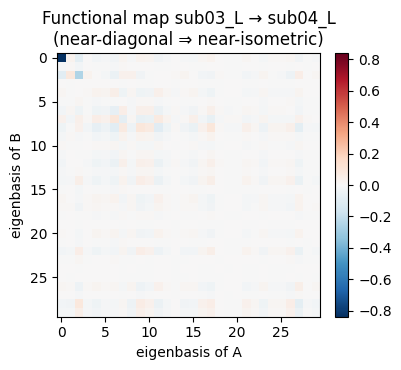
Classical correspondence asks “which point on shape B matches point \(x\) on shape A?” Ovsjanikov et al. (2012) reframed it: instead of mapping points, map functions. A functional map \(C\) is a small matrix that converts the eigenbasis coefficients of a function on A into those on B:
For (near-)isometric shapes, \(C\) is nearly diagonal, because matching eigenfunctions carry matching information. The further from isometric, the more \(C\) spreads off-diagonal. We compute \(C\) between two left hippocampi using their HKS fields as soft constraints, and look at its structure.
import sys
from pathlib import Path
sys.path.insert(0, str(Path.cwd()))
import numpy as np, matplotlib.pyplot as plt
import spectralbrain as sb
from _tutorial_utils import data_path

def load_hipp(sid, hemi="L"):
    v, f = sb.load_gifti_surface(
        data_path("hippunfold", sid, f"hemi-{hemi}_space-T1w_den-8k_label-hipp_midthickness.surf.gii"))
    return sb.BrainMesh(v, f)

A, B = load_hipp("sub03"), load_hipp("sub04")
decA, decB = A.decompose(k=80), B.decompose(k=80)
hksA = np.asarray(sb.compute_hks(decA, n_times=20))
hksB = np.asarray(sb.compute_hks(decB, n_times=20))
pairs = [(hksA[:, j], hksB[:, j]) for j in range(hksA.shape[1])]

C = sb.compute_functional_map(decA, decB, n_basis=30, descriptor_pairs=pairs)
print(f"functional map C: {C.shape}")

fig, ax = plt.subplots(figsize=(4.2, 3.8))
im = ax.imshow(C, cmap="RdBu_r", vmin=-np.abs(C).max(), vmax=np.abs(C).max())
ax.set_title("Functional map sub03_L → sub04_L\n(near-diagonal ⇒ near-isometric)")
ax.set_xlabel("eigenbasis of A"); ax.set_ylabel("eigenbasis of B")
plt.colorbar(im, fraction=0.046); plt.tight_layout(); plt.show()
[06/09/26 02:09:05] INFO Laplacian (cotangent): N=8192, nnz=56578
[06/09/26 02:09:06] INFO Laplacian (cotangent): N=8192, nnz=56578
functional map C: (30, 30)
2. Intrinsic distances: travelling along the shape#
How far apart are two points measured through the structure, not through the air? The spectrum gives several such distances, each weighting eigenmodes differently:
Commute-time distance: expected round-trip time of a random walk between two points, \(d_C(x,y)^2 = \sum_{k\ge1}\frac{1}{\lambda_k}(\varphi_k(x)-\varphi_k(y))^2\).
Biharmonic distance: like commute-time but weighted by \(1/\lambda_k^2\), emphasising global structure and giving smoother fields.
Diffusion distance at time \(t\): \(\sum_k e^{-2\lambda_k t}(\varphi_k(x)-\varphi_k(y))^2\), a scale-tunable distance.
We compute each as a field from one source vertex to all others (passing a single source index avoids the full \(N\times N\) matrix) and render them.
src = int(np.argmax(A.vertices[:, 0]))      # a vertex at one end (hippocampal head/tail)
idx = np.array([src])
d_bih = np.asarray(sb.biharmonic_distance(decA, indices=idx)).ravel()
d_com = np.asarray(sb.commute_time_distance(decA, indices=idx, warn_large=False)).ravel()
d_dif = np.asarray(sb.diffusion_distance(decA, t=10.0, indices=idx)).ravel()

V = A.vertices
fig = plt.figure(figsize=(11, 3.3))
for i, (d, ttl) in enumerate([(d_bih, "biharmonic"), (d_com, "commute-time"), (d_dif, "diffusion (t=10)")]):
    ax = fig.add_subplot(1, 3, i + 1, projection="3d")
    ax.scatter(V[:, 0], V[:, 1], V[:, 2], c=d, cmap="viridis", s=2)
    ax.scatter(*V[src], c="red", s=40)
    ax.set_title(f"{ttl} distance from source", fontsize=9); ax.set_axis_off(); ax.view_init(20, -70)
plt.tight_layout(); plt.show()
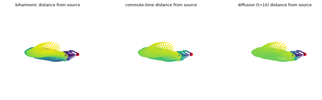
All three grow smoothly away from the red source along the hippocampal body — they respect the intrinsic geometry. Because they are built from the spectrum, they are pose-invariant: rotating the hippocampus leaves them unchanged. Render the biharmonic field with the six-view tool for a publication-quality view.
from spectralbrain.viz import plot_surface_sixview
fig = plot_surface_sixview(A, scalars=d_bih, cmap="viridis",
                           scalar_bar_title="biharmonic dist.",
                           title="Biharmonic distance from a source vertex")
plt.show()
2026-06-09 02:09:08.638 ( 0.261s) [ 7F3F44963080]vtkXOpenGLRenderWindow.:1460 WARN| bad X server connection. DISPLAY=

3. Point-set distances: how far apart in space#
Sometimes we want the opposite: how far two surfaces sit as point sets in the scanner. Chamfer (average nearest-neighbour distance) and Hausdorff (worst-case nearest-neighbour distance) answer this. Unlike everything spectral, they are extrinsic: move one shape and the distance changes. We show this directly by rotating a hippocampus and watching Chamfer rise, while its spectrum (notebook 1) would not have budged.
PA, PB = A.vertices, B.vertices
print(f"sub03_L vs sub04_L  | Chamfer: {sb.chamfer_distance(PA, PB):.3f}  "
      f"Hausdorff: {sb.hausdorff_distance(PA, PB):.3f}")

# Rotate A by 30 degrees about z and recompute — extrinsic distances change.
th = np.deg2rad(30); Rz = np.array([[np.cos(th), -np.sin(th), 0],
                                    [np.sin(th), np.cos(th), 0], [0, 0, 1]])
PA_rot = PA @ Rz.T
print(f"sub03_L (rotated) vs sub04_L | Chamfer: {sb.chamfer_distance(PA_rot, PB):.3f}  "
      f"Hausdorff: {sb.hausdorff_distance(PA_rot, PB):.3f}")
print("\nExtrinsic distances move with pose; spectral descriptors and intrinsic "
      "distances do not. That invariance is the reason to work in the spectrum.")
sub03_L vs sub04_L  | Chamfer: 780.459  Hausdorff: 30.820
sub03_L (rotated) vs sub04_L | Chamfer: 1000.229  Hausdorff: 40.244

Extrinsic distances move with pose; spectral descriptors and intrinsic distances do not. That invariance is the reason to work in the spectrum.
4. Comparing descriptor distributions#
A fourth notion of distance compares the distributions of a descriptor across
two shapes, ignoring point correspondence. descriptor_distance offers Wasserstein
(optimal transport), MMD, and simpler metrics. We compare the HKS distributions of
the two hippocampi.
for method in ["wasserstein", "euclidean", "cosine"]:
    d = sb.descriptor_distance(hksA.mean(0), hksB.mean(0), method=method)
    print(f"  HKS distribution distance ({method:11s}): {d:.4f}")
  HKS distribution distance (wasserstein): 0.0008
  HKS distribution distance (euclidean  ): 0.0008
  HKS distribution distance (cosine     ): 0.0000
Exercises#
Isometry test. Build the functional map from a hippocampus to itself after a random rotation. The map should be (almost) the identity. Is it?
Weighting matters. Overlay the biharmonic and commute-time fields from the same source along one axis of the hippocampus. Which is smoother, and why (think \(1/\lambda_k\) vs \(1/\lambda_k^2\))?
Diffusion scale. Recompute the diffusion distance for
tin[1, 10, 100]. How does the field’s spatial extent change witht?Symmetry of Hausdorff. Compare
hausdorff_distance(A, B, symmetric=False)in both directions. When are they different?Intrinsic vs extrinsic. Rotate
sub03_Land recompute (a) its ShapeDNA distance tosub04_Land (b) its Chamfer distance. Confirm only the extrinsic one changes.
What’s next#
Single-structure analysis is behind us. Notebook 08 scales up to a cohort:
loading groups with load_group, then vertex-wise statistics with proper
family-wise error control (max-statistic permutation, FDR, TFCE) and Cohen’s d
maps. From here the series turns from geometry to inference.