08 · Cohorts & vertex-wise statistics#
SpectralBrain tutorial series — notebook 8 of 10. (Previous: functional maps & distances.)
The series now turns from geometry to inference. We load a cohort with
load_group, then test where a descriptor differs across the surface, with honest
control of the multiple-comparisons problem: max-statistic permutation (family-wise
error), false-discovery control, and threshold-free cluster enhancement.
Learning objectives#
Assemble a cohort into a
GroupDataobject withload_group.Understand why vertex-wise testing needs multiple-comparison correction.
Apply
vertexwise_ttest(FDR),vertexwise_permutation(FWE),cohens_d_map, andtfce.
Note on sample size. This teaching dataset has only a handful of real subjects, far too few for a real group contrast. Sections 1 loads the real cohort to show the machinery; sections 3–5 then use a clearly-labelled synthetic cohort built on the real template geometry, with a planted effect, so the statistics have something to find. Synthetic data is used only to demonstrate the methods, never to make a scientific claim.
1. Loading a cohort#
load_group takes a set of inputs and returns a GroupData. With
mode='pipeline' it runs the spectral pipeline on each subject and stacks the
result. HippUnfold den-8k surfaces share a common topology, so their vertices
correspond across subjects, which is exactly what vertex-wise statistics require.
import sys
from pathlib import Path
sys.path.insert(0, str(Path.cwd()))
import numpy as np, matplotlib.pyplot as plt
import scipy.sparse as sp
import spectralbrain as sb
import spectralbrain.statistics as st
from _tutorial_utils import data_path

files = {f"{s}_{h}": data_path("hippunfold", s,
            f"hemi-{h}_space-T1w_den-8k_label-hipp_midthickness.surf.gii")
         for s in ["sub03", "sub04"] for h in ["L", "R"]}
group = sb.load_group(files, mode="pipeline", descriptor="shapedna", k=60)
print(f"GroupData: {group.n_subjects} subjects, descriptor matrix {group.data.shape}")
print(f"subjects: {group.subject_ids}")
[06/09/26 02:11:02] INFO Laplacian (cotangent): N=8192, nnz=56578
[06/09/26 02:11:03] INFO Laplacian (cotangent): N=8192, nnz=56578
INFO Laplacian (cotangent): N=8192, nnz=56578
[06/09/26 02:11:04] INFO Laplacian (cotangent): N=8192, nnz=56578
[06/09/26 02:11:04] INFO Loaded group: 4/4 subjects (mode=pipeline).
GroupData: 4 subjects, descriptor matrix (4, 59)
subjects: ['sub03_L', 'sub03_R', 'sub04_L', 'sub04_R']
2. The multiple-comparisons problem#
A den-8k hippocampus has ~8,000 vertices. Testing each independently at
\(\alpha=0.05\) would yield ~400 false positives by chance alone. Three standard
remedies, all in SpectralBrain:
FDR (Benjamini–Hochberg): controls the expected proportion of false positives among the rejections. Most sensitive, weakest guarantee.
FWE by max-statistic permutation (Nichols & Holmes 2002): controls the probability of any false positive, by comparing each vertex to the null distribution of the maximum statistic over the whole surface. Strong guarantee.
TFCE (Smith & Nichols 2009): enhances spatially contiguous signal without a hard cluster threshold, then tested by permutation.
We build a template-based synthetic cohort to see them work.
# Real template geometry: a left hippocampus and its HKS field.
mesh = sb.BrainMesh(*sb.load_gifti_surface(files["sub03_L"]))
dec = mesh.decompose(k=200)
template = np.asarray(sb.compute_hks(dec, n_times=100))[:, 60]   # one HKS scale, per vertex
template = (template - template.mean()) / template.std()
N = mesh.n_vertices

# Plant a focal effect at one end of the hippocampus (e.g. the head).
head = mesh.vertices[:, 0] > np.percentile(mesh.vertices[:, 0], 80)
print(f"planted-effect region: {head.sum()} of {N} vertices")

rng = np.random.default_rng(42)
n_per = 16
A = template[None, :] + rng.normal(0, 1.0, (n_per, N))            # controls
B = template[None, :] + rng.normal(0, 1.0, (n_per, N))            # patients
B[:, head] += 1.2                                                 # focal group difference
print(f"synthetic cohort: group A {A.shape}, group B {B.shape}  (SYNTHETIC — teaching only)")
[06/09/26 02:11:05] INFO Laplacian (cotangent): N=8192, nnz=56578
planted-effect region: 1639 of 8192 vertices
synthetic cohort: group A (16, 8192), group B (16, 8192)  (SYNTHETIC — teaching only)
3. Three corrections, compared#
We run the parametric \(t\)-test with FDR, the permutation test with FWE max-stat control, and read off how many vertices each declares significant. FWE is the most conservative; FDR the most permissive; both should localise to the planted head region.
res_fdr = st.vertexwise_ttest(A, B, correction="fdr", alpha=0.05)
res_fwe = st.vertexwise_permutation(A, B, n_permutations=2000, correction="max", seed=0, alpha=0.05)
d_map = np.asarray(st.cohens_d_map(A, B))

print(f"FDR  significant vertices: {int(res_fdr.n_significant):4d}")
print(f"FWE  significant vertices: {int(res_fwe.n_significant):4d}")
print(f"max |Cohen's d|: {np.abs(d_map).max():.2f}  "
      f"(planted region mean d = {d_map[head].mean():.2f}, elsewhere = {d_map[~head].mean():.2f})")

# fraction of detections that fall inside the planted region (precision)
for name, res in [("FDR", res_fdr), ("FWE", res_fwe)]:
    sigv = np.asarray(res.significant)
    if sigv.sum():
        print(f"  {name}: {100*sigv[head].sum()/sigv.sum():.0f}% of significant vertices lie in the planted region")
FDR  significant vertices: 1214
FWE  significant vertices:   88
max |Cohen's d|: 2.67  (planted region mean d = -1.25, elsewhere = -0.00)
  FDR: 96% of significant vertices lie in the planted region
  FWE: 100% of significant vertices lie in the planted region
4. TFCE: cluster-free spatial enhancement#
TFCE boosts vertices that sit in spatially extended regions of signal, using the mesh adjacency. We build adjacency from the surface faces and enhance the \(t\)-map.
F = mesh.faces
rows = np.concatenate([F[:, 0], F[:, 1], F[:, 2], F[:, 1], F[:, 2], F[:, 0]])
cols = np.concatenate([F[:, 1], F[:, 2], F[:, 0], F[:, 0], F[:, 1], F[:, 2]])
adj = sp.csr_matrix((np.ones(len(rows)), (rows, cols)), shape=(N, N))
adj = (adj > 0).astype(float)

tfce_map = np.asarray(st.tfce(res_fwe.statistic, adj))
print(f"TFCE map: range {tfce_map.min():.2f} .. {tfce_map.max():.2f}")
print(f"TFCE signal concentrated in planted region? "
      f"mean inside={tfce_map[head].mean():.2f} vs outside={tfce_map[~head].mean():.2f}")
TFCE map: range 0.00 .. 537.41
TFCE signal concentrated in planted region? mean inside=284.31 vs outside=8.01
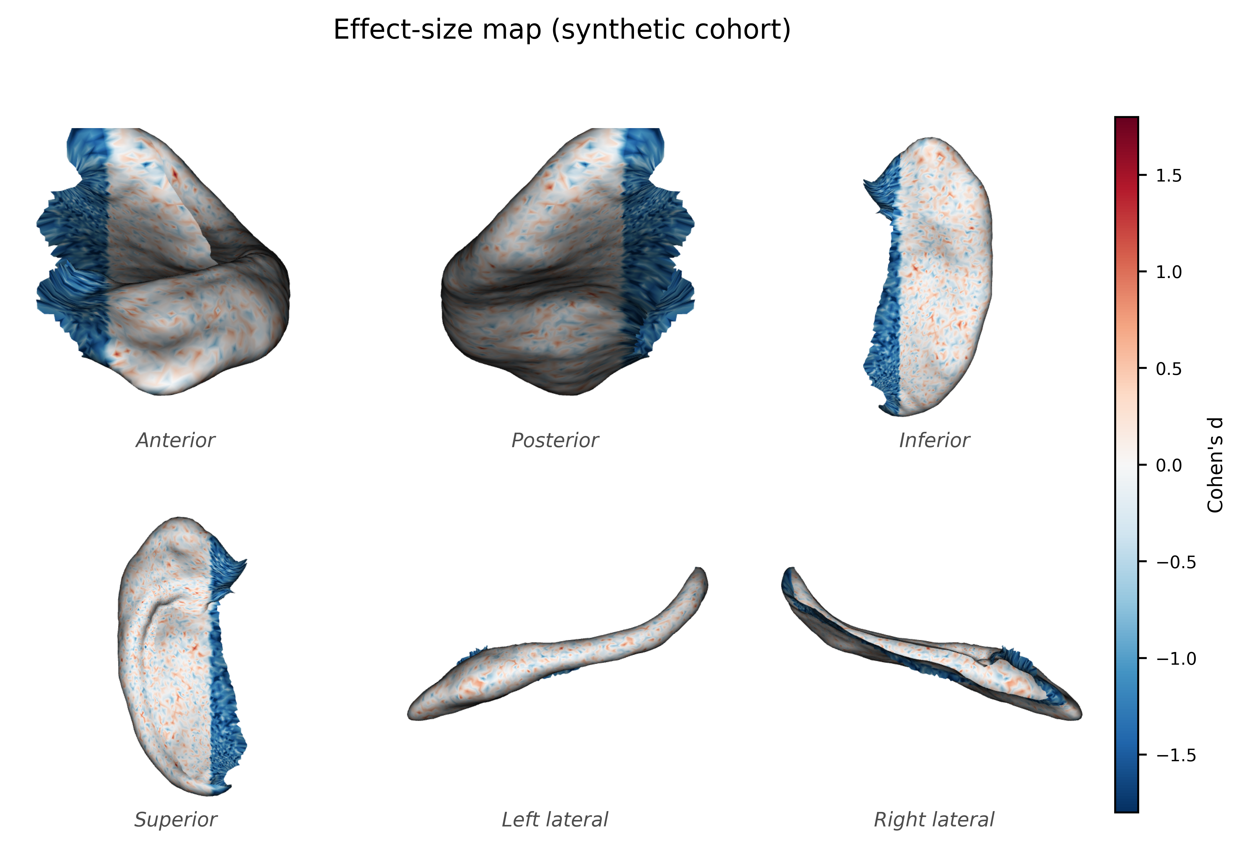
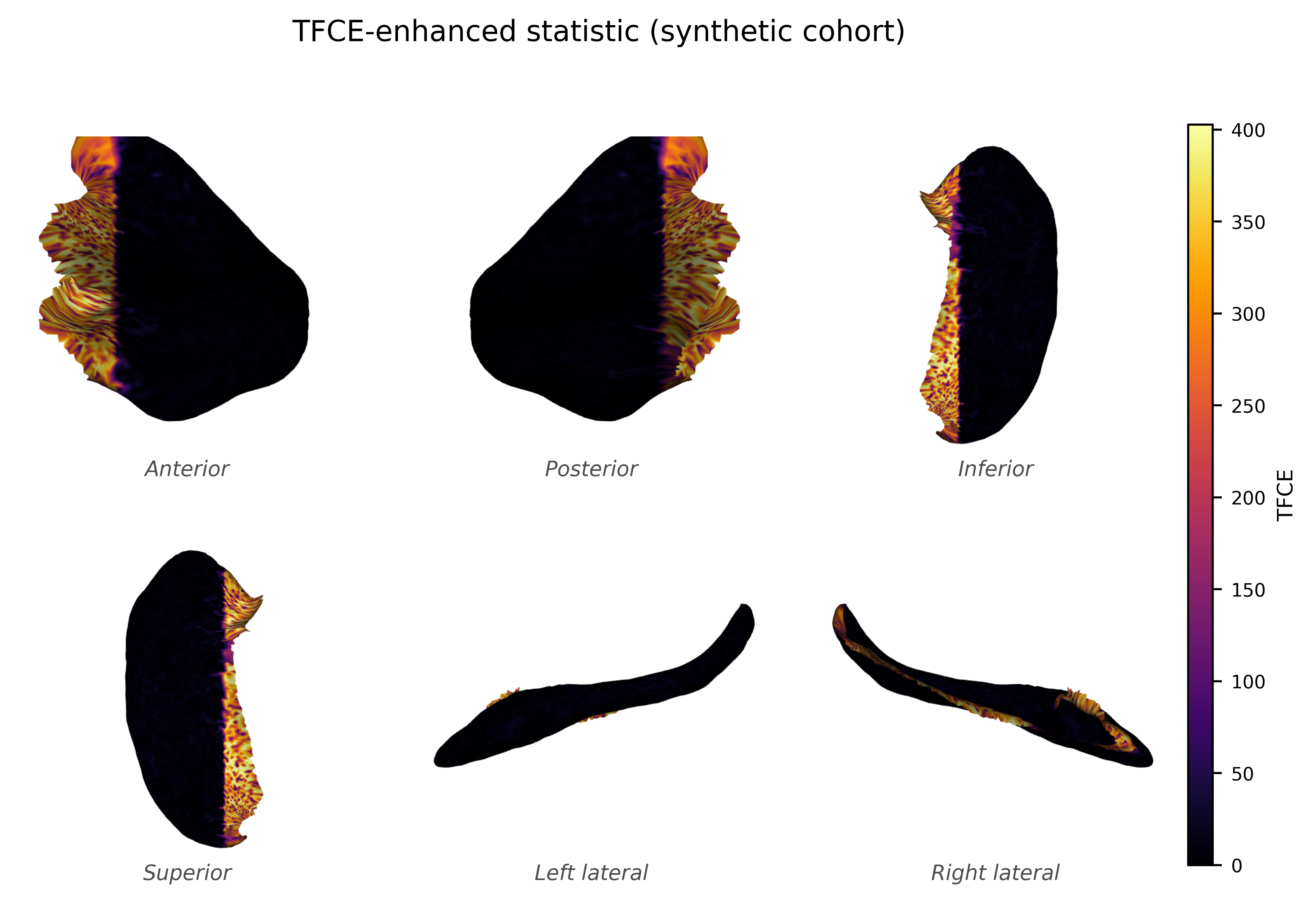
5. Mapping the result#
The whole point of vertex-wise analysis is localisation. We render the Cohen’s d map and the TFCE map on the surface with the six-view tool. The signal should light up exactly the planted head region, which is how you would read a real group difference in, say, hippocampal sclerosis.
from spectralbrain.viz import plot_surface_sixview
fig = plot_surface_sixview(mesh, scalars=d_map, cmap="RdBu_r", signed=True,
                           scalar_bar_title="Cohen's d", title="Effect-size map (synthetic cohort)")
plt.show()
fig = plot_surface_sixview(mesh, scalars=tfce_map, cmap="inferno",
                           scalar_bar_title="TFCE", title="TFCE-enhanced statistic (synthetic cohort)")
plt.show()
2026-06-09 02:11:20.145 ( 0.313s) [ 7F69ABDB2080]vtkXOpenGLRenderWindow.:1460 WARN| bad X server connection. DISPLAY=
Exercises#
Effect size vs n. Halve the planted effect (
+0.6instead of+1.2) and re-run. Which correction still detects it — FDR, FWE, or neither?Where is the signal? Plant the effect in the hippocampal tail (
< 20th percentileof x) instead of the head and confirm the maps follow.Permutation count. Re-run
vertexwise_permutationwith 500 vs 5000 permutations. How stable isn_significant? What does the count buy you?Correlation, not contrast. Use
vertexwise_correlationto relate the per-vertex HKS to a synthetic continuous score across subjects, with FDR.Real cohort. Replace the synthetic data with the four real subjects’ HKS maps (
load_group(..., descriptor='hks')) and a left-vs-right contrast. Why is nothing significant, and what would you need to change?
What’s next#
Vertex-wise maps tell us where. Notebook 09 quantifies how much and how reliably: DeLong’s test for comparing classifier AUCs, bias-corrected bootstrap intervals, intraclass correlation for reliability, cross-validated classification, and multi-site harmonisation with ComBat.